API
Introduction
This section describes application programming interface (API) for the fuc package.
Below is the list of submodules available in the fuc API:
common : The common submodule is used by other fuc submodules such as pyvcf and pybed. It also provides many day-to-day actions used in the field of bioinformatics.
pybam : The pybam submodule is designed for working with sequence alignment files (SAM/BAM/CRAM). It essentially wraps the pysam package to allow fast computation and easy manipulation. If you are mainly interested in working with depth of coverage data, please check out the pycov submodule which is specifically designed for the task.
pybed : The pybed submodule is designed for working with BED files. It implements
pybed.BedFramewhich stores BED data aspandas.DataFramevia the pyranges package to allow fast computation and easy manipulation. The submodule strictly adheres to the standard BED specification.pychip : The pychip submodule is designed for working with annotation or manifest files from the Axiom (Thermo Fisher Scientific) and Infinium (Illumina) array platforms.
pycov : The pycov submodule is designed for working with depth of coverage data from sequence alingment files (SAM/BAM/CRAM). It implements
pycov.CovFramewhich stores read depth data aspandas.DataFramevia the pysam package to allow fast computation and easy manipulation. Thepycov.CovFrameclass also contains many useful plotting methods such asCovFrame.plot_regionandCovFrame.plot_uniformity.pyfq : The pyfq submodule is designed for working with FASTQ files. It implements
pyfq.FqFramewhich stores FASTQ data aspandas.DataFrameto allow fast computation and easy manipulation.pygff : The pygff submodule is designed for working with GFF/GTF files. It implements
pygff.GffFramewhich stores GFF/GTF data aspandas.DataFrameto allow fast computation and easy manipulation. The submodule strictly adheres to the standard GFF specification.pykallisto : The pykallisto submodule is designed for working with RNAseq quantification data from Kallisto. It implements
pykallisto.KallistoFramewhich stores Kallisto’s output data aspandas.DataFrameto allow fast computation and easy manipulation. Thepykallisto.KallistoFrameclass also contains many useful plotting methods such asKallistoFrame.plot_differential_abundance.pymaf : The pymaf submodule is designed for working with MAF files. It implements
pymaf.MafFramewhich stores MAF data aspandas.DataFrameto allow fast computation and easy manipulation. Thepymaf.MafFrameclass also contains many useful plotting methods such asMafFrame.plot_oncoplotandMafFrame.plot_summary. The submodule strictly adheres to the standard MAF specification.pysnpeff : The pysnpeff submodule is designed for parsing VCF annotation data from the SnpEff program. It should be used with
pyvcf.VcfFrame.pyvcf : The pyvcf submodule is designed for working with VCF files. It implements
pyvcf.VcfFramewhich stores VCF data aspandas.DataFrameto allow fast computation and easy manipulation. Thepyvcf.VcfFrameclass also contains many useful plotting methods such asVcfFrame.plot_comparisonandVcfFrame.plot_tmb. The submodule strictly adheres to the standard VCF specification.pyvep : The pyvep submodule is designed for parsing VCF annotation data from the Ensembl VEP program. It should be used with
pyvcf.VcfFrame.
For getting help on a specific submodule (e.g. pyvcf):
from fuc import pyvcf
help(pyvcf)
fuc.common
The common submodule is used by other fuc submodules such as pyvcf and pybed. It also provides many day-to-day actions used in the field of bioinformatics.
Classes:
|
Class for storing sample annotation data. |
Functions:
|
Print colored text. |
str : Name of the current conda environment. |
|
Convert a text file to a list of filenames. |
|
|
Convert numeric values to categorical variables. |
|
Extract the DNA sequence corresponding to a selected region from a FASTA file. |
|
Return the most similar string in a list. |
|
Return a value from 0 to 1 representing how similar two strings are. |
|
Return True if the similarity is equal to or greater than threshold. |
|
Create custom legend handles. |
|
Load an example dataset from the online repository (requires internet). |
|
Parse the input variable and then return a list of items. |
|
Parse specified genomic region. |
|
Parse specified genomic variant. |
|
Create a gene model where exons are drawn as boxes. |
|
Rename sample names flexibly. |
|
Given a DNA sequence, generate its reverse, complement, or reverse-complement. |
|
Return sorted list of regions. |
|
Return sorted list of variants. |
|
Return various summary statistics from (FP, FN, TP, TN). |
|
Add or remove the (annoying) 'chr' string from specified regions. |
- class fuc.api.common.AnnFrame(df)[source]
Class for storing sample annotation data.
This class stores sample annotation data as
pandas.DataFramewith sample names as index.Note that an AnnFrame can have a different set of samples than its accompanying
pymaf.MafFrame,pyvcf.VcfFrame, etc.- Parameters:
df (pandas.DataFrame) – DataFrame containing sample annotation data. The index must be unique sample names.
See also
AnnFrame.from_dictConstruct AnnFrame from dict of array-like or dicts.
AnnFrame.from_fileConstruct AnnFrame from a delimited text file.
Examples
>>> import pandas as pd
>>> from fuc import common
>>> data = {
...     'SampleID': ['A', 'B', 'C', 'D'],
...     'PatientID': ['P1', 'P1', 'P2', 'P2'],
...     'Tissue': ['Normal', 'Tissue', 'Normal', 'Tumor'],
...     'Age': [30, 30, 57, 57]
... }
>>> df = pd.DataFrame(data)
>>> df = df.set_index('SampleID')
>>> af = common.AnnFrame(df)
>>> af.df
         PatientID  Tissue  Age
SampleID
A               P1  Normal   30
B               P1  Tissue   30
C               P2  Normal   57
D               P2   Tumor   57
Attributes:
DataFrame containing sample annotation data.
List of the sample names.
Dimensionality of AnnFrame (samples, annotations).
Methods:
from_dict(data, sample_col)Construct AnnFrame from dict of array-like or dicts.
from_file(fn, sample_col[, sep])Construct AnnFrame from a delimited text file.
plot_annot(group_col[, group_order, ...])Create a categorical heatmap for the selected column using unmatched samples.
plot_annot_matched(patient_col, group_col, ...)Create a categorical heatmap for the selected column using matched samples.
sorted_samples(by[, mf, keep_empty, nonsyn])Return a sorted list of sample names.
subset(samples[, exclude])Subset AnnFrame for specified samples.
- property df
DataFrame containing sample annotation data.
- Type:
pandas.DataFrame
- classmethod from_dict(data, sample_col)[source]
Construct AnnFrame from dict of array-like or dicts.
The dictionary must contain a column that represents sample names.
- Parameters:
data (dict) – Of the form {field : array-like} or {field : dict}.
sample_col (str or int) – Column containing unique sample names, either given as string name or column index.
- Returns:
AnnFrame object.
- Return type:
See also
AnnFrameAnnFrame object creation using constructor.
AnnFrame.from_fileConstruct AnnFrame from a delimited text file.
Examples
>>> from fuc import common
>>> data = {
...     'SampleID': ['A', 'B', 'C', 'D'],
...     'PatientID': ['P1', 'P1', 'P2', 'P2'],
...     'Tissue': ['Normal', 'Tissue', 'Normal', 'Tumor'],
...     'Age': [30, 30, 57, 57]
... }
>>> af = common.AnnFrame.from_dict(data, sample_col='SampleID') # or sample_col=0
>>> af.df
         PatientID  Tissue  Age
SampleID
A               P1  Normal   30
B               P1  Tissue   30
C               P2  Normal   57
D               P2   Tumor   57
- classmethod from_file(fn, sample_col, sep='\t')[source]
Construct AnnFrame from a delimited text file.
The file must contain a column that represents sample names.
- Parameters:
fn (str) – Text file (compressed or uncompressed).
sample_col (str or int) – Column containing unique sample names, either given as string name or column index.
sep (str, default: ‘\t’) – Delimiter to use.
- Returns:
AnnFrame object.
- Return type:
See also
AnnFrameAnnFrame object creation using constructor.
AnnFrame.from_dictConstruct AnnFrame from dict of array-like or dicts.
Examples
>>> from fuc import common
>>> af = common.AnnFrame.from_file('sample-annot.tsv', sample_col='SampleID')
>>> af = common.AnnFrame.from_file('sample-annot.csv', sample_col=0, sep=',')
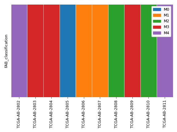
- plot_annot(group_col, group_order=None, samples=None, colors='tab10', sequential=False, xticklabels=True, ax=None, figsize=None)[source]
Create a categorical heatmap for the selected column using unmatched samples.
See this tutorial to learn how to create customized oncoplots.
- Parameters:
group_col (str) – AnnFrame column containing sample group information. If the column has NaN values, they will be converted to ‘N/A’ string.
group_order (list, optional) – List of sample group names (in that order too). You can use this to subset samples belonging to specified groups only. You must include all relevant groups when also using
samples.samples (list, optional) – Display only specified samples (in that order too).
colors (str or list, default: ‘tab10’) – Colormap name or list of colors.
sequential (bool, default: False) – Whether the column is sequential data.
xticklabels (bool, default: True) – If True, plot the sample names.
ax (matplotlib.axes.Axes, optional) – Pre-existing axes for the plot. Otherwise, crete a new one.
figsize (tuple, optional) – Width, height in inches. Format: (float, float).
- Returns:
matplotlib.axes.Axes – The matplotlib axes containing the plot.
list – Legend handles.
Examples
Below is a simple example:
>>> import matplotlib.pyplot as plt
>>> from fuc import common, pymaf
>>> common.load_dataset('tcga-laml')
>>> annot_file = '~/fuc-data/tcga-laml/tcga_laml_annot.tsv'
>>> af = common.AnnFrame.from_file(annot_file, sample_col=0)
>>> ax, handles = af.plot_annot('FAB_classification', samples=af.samples[:10])
>>> legend = ax.legend(handles=handles)
>>> ax.add_artist(legend)
>>> plt.tight_layout()
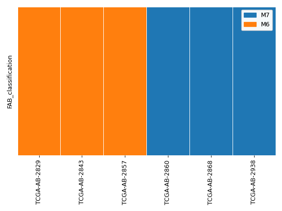
We can display only selected groups:
>>> ax, handles = af.plot_annot('FAB_classification', group_order=['M7', 'M6'])
>>> legend = ax.legend(handles=handles)
>>> ax.add_artist(legend)
>>> plt.tight_layout()
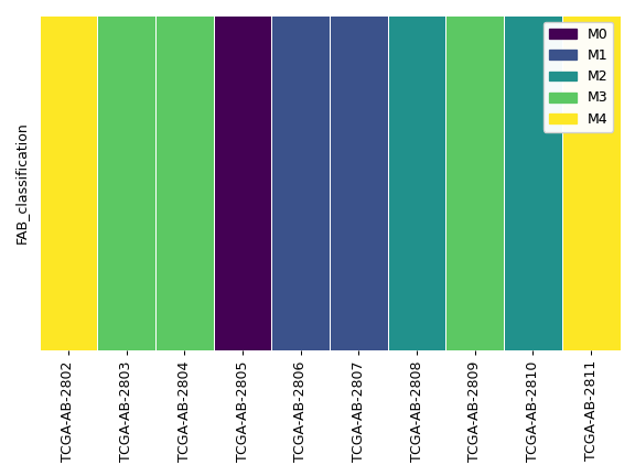
We can also display sequenital data in the following way:
>>> ax, handles = af.plot_annot('FAB_classification',
...                             samples=af.samples[:10],
...                             colors='viridis',
...                             sequential=True)
>>> legend = ax.legend(handles=handles)
>>> ax.add_artist(legend)
>>> plt.tight_layout()
- plot_annot_matched(patient_col, group_col, annot_col, patient_order=None, group_order=None, annot_order=None, colors='tab10', sequential=False, xticklabels=True, ax=None, figsize=None)[source]
Create a categorical heatmap for the selected column using matched samples.
See this tutorial to learn how to create customized oncoplots.
- Parameters:
patient_col (str) – AnnFrame column containing patient information.
group_col (str) – AnnFrame column containing sample group information.
annot_col (str) – Column to plot.
patient_order (list, optional) – Plot only specified patients (in that order too).
group_order (list, optional) – List of sample group names.
annot_order (list, optional) – Plot only specified annotations (in that order too).
colors (str or list, default: ‘tab10’) – Colormap name or list of colors.
sequential (bool, default: False) – Whether the column is sequential data.
xticklabels (bool, default: True) – If True, plot the sample names.
ax (matplotlib.axes.Axes, optional) – Pre-existing axes for the plot. Otherwise, crete a new one.
figsize (tuple, optional) – Width, height in inches. Format: (float, float).
- Returns:
matplotlib.axes.Axes – The matplotlib axes containing the plot.
list – Legend handles.
- property samples
List of the sample names.
- Type:
list
- property shape
Dimensionality of AnnFrame (samples, annotations).
- Type:
tuple
- sorted_samples(by, mf=None, keep_empty=False, nonsyn=False)[source]
Return a sorted list of sample names.
- Parameters:
df (str or list) – Column or list of columns to sort by.
- subset(samples, exclude=False)[source]
Subset AnnFrame for specified samples.
- Parameters:
samples (str or list) – Sample name or list of names (the order matters).
exclude (bool, default: False) – If True, exclude specified samples.
- Returns:
Subsetted AnnFrame.
- Return type:
Examples
>>> from fuc import common
>>> data = {
...     'SampleID': ['A', 'B', 'C', 'D'],
...     'PatientID': ['P1', 'P1', 'P2', 'P2'],
...     'Tissue': ['Normal', 'Tumor', 'Normal', 'Tumor'],
...     'Age': [30, 30, 57, 57]
... }
>>> af = common.AnnFrame.from_dict(data, sample_col='SampleID') # or sample_col=0
>>> af.df
         PatientID  Tissue  Age
SampleID
A               P1  Normal   30
B               P1   Tumor   30
C               P2  Normal   57
D               P2   Tumor   57
We can subset the AnnFrame for the normal samples A and C:
>>> af.subset(['A', 'C']).df
         PatientID  Tissue  Age
SampleID
A               P1  Normal   30
C               P2  Normal   57
Alternatively, we can exclude those samples:
>>> af.subset(['A', 'C'], exclude=True).df
         PatientID Tissue  Age
SampleID
B               P1  Tumor   30
D               P2  Tumor   57
- fuc.api.common.convert_file2list(fn)[source]
Convert a text file to a list of filenames.
- Parameters:
fn (str) – File containing one filename per line.
- Returns:
List of filenames.
- Return type:
list
Examples
>>> from fuc import common
>>> common.convert_file2list('bam.list')
['1.bam', '2.bam', '3.bam']
- fuc.api.common.convert_num2cat(s, n=5, decimals=0)[source]
Convert numeric values to categorical variables.
- Parameters:
pandas.Series – Series object containing numeric values.
n (int, default: 5) – Number of variables to output.
- Returns:
Series object containing categorical variables.
- Return type:
pandas.Series
Examples
>>> import matplotlib.pyplot as plt
>>> from fuc import common, pymaf
>>> common.load_dataset('tcga-laml')
>>> annot_file = '~/fuc-data/tcga-laml/tcga_laml_annot.tsv'
>>> af = common.AnnFrame.from_file(annot_file, sample_col=0)
>>> s = af.df.days_to_last_followup
>>> s[:10]
Tumor_Sample_Barcode
TCGA-AB-2802     365.0
TCGA-AB-2803     792.0
TCGA-AB-2804    2557.0
TCGA-AB-2805     577.0
TCGA-AB-2806     945.0
TCGA-AB-2807     181.0
TCGA-AB-2808    2861.0
TCGA-AB-2809      62.0
TCGA-AB-2810      31.0
TCGA-AB-2811     243.0
Name: days_to_last_followup, dtype: float64
>>> s = common.convert_num2cat(s)
>>> s.unique()
array([ 572.2, 1144.4, 2861. , 2288.8, 1716.6,    nan])
>>> s[:10]
Tumor_Sample_Barcode
TCGA-AB-2802     572.2
TCGA-AB-2803    1144.4
TCGA-AB-2804    2861.0
TCGA-AB-2805    1144.4
TCGA-AB-2806    1144.4
TCGA-AB-2807     572.2
TCGA-AB-2808    2861.0
TCGA-AB-2809     572.2
TCGA-AB-2810     572.2
TCGA-AB-2811     572.2
Name: days_to_last_followup, dtype: float64
- fuc.api.common.extract_sequence(fasta, region)[source]
Extract the DNA sequence corresponding to a selected region from a FASTA file.
The method also allows users to retrieve the reference allele of a variant in a genomic coordinate format, instead of providing a genomic region.
- Parameters:
fasta (str) – FASTA file.
region (str) – Region (‘chrom:start-end’).
- Returns:
DNA sequence. Empty string if there is no matching sequence.
- Return type:
str
Examples
>>> from fuc import common
>>> fasta = 'resources_broad_hg38_v0_Homo_sapiens_assembly38.fasta'
>>> common.extract_sequence(fasta, 'chr1:15000-15005')
'GATCCG'
>>> # rs1423852 is chr16-80874864-C-T
>>> common.extract_sequence(fasta, 'chr16:80874864-80874864')
'C'
- fuc.api.common.get_similarity(a, b)[source]
Return a value from 0 to 1 representing how similar two strings are.
- fuc.api.common.is_similar(a, b, threshold=0.9)[source]
Return True if the similarity is equal to or greater than threshold.
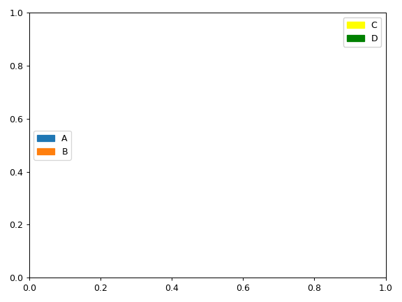
- fuc.api.common.legend_handles(labels, colors='tab10')[source]
Create custom legend handles.
- Parameters:
labels (list) – List of labels.
colors (str or list, default: ‘tab10’) – Colormap name or list of colors.
- Returns:
List of legend handles.
- Return type:
list
Examples
>>> import matplotlib.pyplot as plt
>>> from fuc import common
>>> fig, ax = plt.subplots()
>>> handles1 = common.legend_handles(['A', 'B'], colors='tab10')
>>> handles2 = common.legend_handles(['C', 'D'], colors=['yellow', 'green'])
>>> legend1 = ax.legend(handles=handles1, loc='center left')
>>> legend2 = ax.legend(handles=handles2)
>>> ax.add_artist(legend1)
>>> ax.add_artist(legend2)
>>> plt.tight_layout()
- fuc.api.common.load_dataset(name, force=False)[source]
Load an example dataset from the online repository (requires internet).
- Parameters:
name (str) – Name of the dataset in https://github.com/sbslee/fuc-data.
force (bool, default: False) – If True, overwrite the existing files.
- fuc.api.common.parse_list_or_file(obj, extensions=['txt', 'tsv', 'csv', 'list'])[source]
Parse the input variable and then return a list of items.
This method is useful when parsing a command line argument that accepts either a list of items or a text file containing one item per line.
- Parameters:
obj (str or list) – Object to be tested. Must be non-empty.
extensions (list, default: [‘txt’, ‘tsv’, ‘csv’, ‘list’]) – Recognized file extensions.
- Returns:
List of items.
- Return type:
list
Examples
>>> from fuc import common
>>> common.parse_list_or_file(['A', 'B', 'C'])
['A', 'B', 'C']
>>> common.parse_list_or_file('A')
['A']
>>> common.parse_list_or_file('example.txt')
['A', 'B', 'C']
>>> common.parse_list_or_file(['example.txt'])
['A', 'B', 'C']
- fuc.api.common.parse_region(region)[source]
Parse specified genomic region.
The method will return parsed region as a tuple with a shape of
(chrom, start, end)which has data types of(str, int, int).Note that only
chromis required when specifing a region. Ifstartandendare omitted, the method will returnNaNin their respective positions in the output tuple.- Parameters:
region (str) – Region (‘chrom:start-end’).
- Returns:
Parsed region.
- Return type:
tuple
Examples
>>> from fuc import common
>>> common.parse_region('chr1:100-150')
('chr1', 100, 150)
>>> common.parse_region('chr1')
('chr1', nan, nan)
>>> common.parse_region('chr1:100')
('chr1', 100, nan)
>>> common.parse_region('chr1:100-')
('chr1', 100, nan)
>>> common.parse_region('chr1:-100')
('chr1', nan, 100)
- fuc.api.common.parse_variant(variant)[source]
Parse specified genomic variant.
Generally speaking, the input string should consist of chromosome, position, reference allele, and alternative allele separated by any one or combination of the following delimiters:
-,:,>(e.g. ‘22-42127941-G-A’). The method will return parsed variant as a tuple with a shape of(chrom, pos, ref, alt)which has data types of(str, int, str, str).Note that it’s possible to omit reference allele and alternative allele from the input string to indicate position-only data (e.g. ‘22-42127941’). In this case, the method will return empty string for the alleles – i.e.
(str, int, '', '')if both are omitted and(str, int, str, '')if only alternative allele is omitted.- Parameters:
variant (str) – Genomic variant.
- Returns:
Parsed variant.
- Return type:
tuple
Examples
>>> from fuc import common
>>> common.parse_variant('22-42127941-G-A')
('22', 42127941, 'G', 'A')
>>> common.parse_variant('22:42127941-G>A')
('22', 42127941, 'G', 'A')
>>> common.parse_variant('22-42127941')
('22', 42127941, '', '')
>>> common.parse_variant('22-42127941-G')
('22', 42127941, 'G', '')
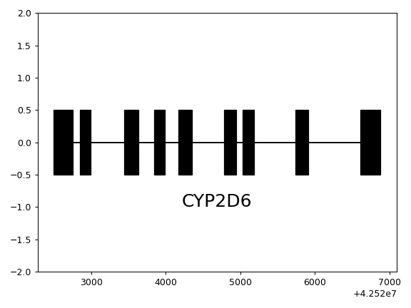
- fuc.api.common.plot_exons(starts, ends, name=None, offset=1, fontsize=None, color='black', y=0, height=1, ax=None, figsize=None)[source]
Create a gene model where exons are drawn as boxes.
- Parameters:
starts (list) – List of exon start positions.
ends (list) – List of exon end positions.
name (str, optional) – Gene name. Use
name='$text$'to italicize the text.offset (float, default: 1) – How far gene name should be plotted from the gene model.
color (str, default: ‘black’) – Box color.
y (float, default: 0) – Y position of the backbone.
height (float, default: 1) – Height of the gene model.
ax (matplotlib.axes.Axes, optional) – Pre-existing axes for the plot. Otherwise, crete a new one.
figsize (tuple, optional) – Width, height in inches. Format: (float, float).
- Returns:
The matplotlib axes containing the plot.
- Return type:
matplotlib.axes.Axes
Examples
>>> import matplotlib.pyplot as plt
>>> from fuc import common
>>> cyp2d6_starts = [42522500, 42522852, 42523448, 42523843, 42524175, 42524785, 42525034, 42525739, 42526613]
>>> cyp2d6_ends = [42522754, 42522994, 42523636, 42523985, 42524352, 42524946, 42525187, 42525911, 42526883]
>>> ax = common.plot_exons(cyp2d6_starts, cyp2d6_ends, name='CYP2D6', fontsize=20)
>>> ax.set_ylim([-2, 2])
>>> plt.tight_layout()
- fuc.api.common.rename(original, names, indicies=None)[source]
Rename sample names flexibly.
- Parameters:
original (list) – List of original names.
names (dict or list) – Dict of old names to new names or list of new names.
indicies (list or tuple, optional) – List of 0-based sample indicies. Alternatively, a tuple (int, int) can be used to specify an index range.
- Returns:
List of updated names.
- Return type:
list
Examples
>>> from fuc import common
>>> original = ['A', 'B', 'C', 'D']
>>> common.rename(original, ['1', '2', '3', '4'])
['1', '2', '3', '4']
>>> common.rename(original, {'B': '2', 'C': '3'})
['A', '2', '3', 'D']
>>> common.rename(original, ['2', '4'], indicies=[1, 3])
['A', '2', 'C', '4']
>>> common.rename(original, ['2', '3'], indicies=(1, 3))
['A', '2', '3', 'D']
- fuc.api.common.reverse_complement(seq, complement=True, reverse=False)[source]
Given a DNA sequence, generate its reverse, complement, or reverse-complement.
- Parameters:
seq (str) – DNA sequence.
complement (bool, default: True) – Whether to return the complment.
reverse (bool, default: False) – Whether to return the reverse.
- Returns:
Updated sequence.
- Return type:
str
Examples
>>> from fuc import common
>>> common.reverse_complement('AGC')
'TCG'
>>> common.reverse_complement('AGC', reverse=True)
'GCT'
>>> common.reverse_complement('AGC', reverse=True, complement=False)
'GCT'
>>> common.reverse_complement('agC', reverse=True)
'Gct'
- fuc.api.common.sort_regions(regions)[source]
Return sorted list of regions.
- Parameters:
regions (list) – List of regions.
- Returns:
Sorted list.
- Return type:
list
Examples
>>> from fuc import common
>>> regions = ['chr22:1000-1500', 'chr16:100-200', 'chr22:200-300', 'chr16_KI270854v1_alt', 'chr3_GL000221v1_random', 'HLA-A*02:10']
>>> sorted(regions) # Lexicographic sorting (not what we want)
['HLA-A*02:10', 'chr16:100-200', 'chr16_KI270854v1_alt', 'chr22:1000-1500', 'chr22:200-300', 'chr3_GL000221v1_random']
>>> common.sort_regions(regions)
['chr16:100-200', 'chr22:200-300', 'chr22:1000-1500', 'chr16_KI270854v1_alt', 'chr3_GL000221v1_random', 'HLA-A*02:10']
- fuc.api.common.sort_variants(variants)[source]
Return sorted list of variants.
- Parameters:
variants (list) – List of variants.
- Returns:
Sorted list.
- Return type:
list
Examples
>>> from fuc import common
>>> variants = ['5-200-G-T', '5:100:T:C', '1:100:A>C', '10-100-G-C']
>>> sorted(variants) # Lexicographic sorting (not what we want)
['10-100-G-C', '1:100:A>C', '5-200-G-T', '5:100:T:C']
>>> common.sort_variants(variants)
['1:100:A>C', '5:100:T:C', '5-200-G-T', '10-100-G-C']
- fuc.api.common.sumstat(fp, fn, tp, tn)[source]
Return various summary statistics from (FP, FN, TP, TN).
This method will return the following statistics:
Terminology
Derivation
sensitivity, recall, hit rate, or true positive rate (TPR)
\(TPR = TP / P = TP / (TP + FN) = 1 - FNR\)
specificity, selectivity or true negative rate (TNR)
\(TNR = TN / N = TN / (TN + FP) = 1 - FPR\)
precision or positive predictive value (PPV)
\(PPV = TP / (TP + FP) = 1 - FDR\)
negative predictive value (NPV)
\(NPV = TN / (TN + FN) = 1 - FOR\)
miss rate or false negative rate (FNR)
\(FNR = FN / P = FN / (FN + TP) = 1 - TPR\)
fall-out or false positive rate (FPR)
\(FPR = FP / N = FP / (FP + TN) = 1 - TNR\)
false discovery rate (FDR)
\(FDR = FP / (FP + TP) = 1 - PPV\)
false omission rate (FOR)
\(FOR = FN / (FN + TN) = 1 - NPV\)
accuracy (ACC)
\(ACC = (TP + TN)/(TP + TN + FP + FN)\)
- Parameters:
fp, fn, tp, tn (int) – Input statistics.
- Returns:
Dictionary containing summary statistics.
- Return type:
dict
Examples
This example is directly taken from the Wiki page Sensitivity and specificity.
>>> from fuc import common
>>> results = common.sumstat(180, 10, 20, 1820)
>>> for k, v in results.items():
...     print(k, f'{v:.3f}')
...
tpr 0.667
tnr 0.910
ppv 0.100
npv 0.995
fnr 0.333
fpr 0.090
fdr 0.900
for 0.005
acc 0.906
- fuc.api.common.update_chr_prefix(regions, mode='remove')[source]
Add or remove the (annoying) ‘chr’ string from specified regions.
The method will automatically detect regions that don’t need to be updated and will return them unchanged.
- Parameters:
regions (str or list) – One or more regions to be updated.
mode ({‘add’, ‘remove’}, default: ‘remove’) – Whether to add or remove the ‘chr’ string.
- Returns:
str or list.
- Return type:
Example
>>> from fuc import common
>>> common.update_chr_prefix(['chr1:100-200', '2:300-400'], mode='remove')
['1:100-200', '2:300-400']
>>> common.update_chr_prefix(['chr1:100-200', '2:300-400'], mode='add')
['chr1:100-200', 'chr2:300-400']
>>> common.update_chr_prefix('chr1:100-200', mode='remove')
'1:100-200'
>>> common.update_chr_prefix('chr1:100-200', mode='add')
'chr1:100-200'
>>> common.update_chr_prefix('2:300-400', mode='add')
'chr2:300-400'
>>> common.update_chr_prefix('2:300-400', mode='remove')
'2:300-400'
fuc.pybam
The pybam submodule is designed for working with sequence alignment files (SAM/BAM/CRAM). It essentially wraps the pysam package to allow fast computation and easy manipulation. If you are mainly interested in working with depth of coverage data, please check out the pycov submodule which is specifically designed for the task.
Functions:
|
Count allelic depth for specified sites. |
|
Return True if contigs have the (annoying) 'chr' string. |
|
Index a BAM file. |
|
Slice a BAM file for specified regions. |
|
Extract SM tags (sample names) from a BAM file. |
|
Extract SN tags (contig names) from a BAM file. |
- fuc.api.pybam.count_allelic_depth(bam, sites)[source]
Count allelic depth for specified sites.
- Parameters:
bam (str) – BAM file.
sites (str or list) – Genomic site or list of sites. Each site should consist of chromosome and 1-based position in the format that can be recognized by
common.parse_variant()(e.g. ‘22-42127941’).
- Returns:
DataFrame containing allelic depth.
- Return type:
pandas.DataFrame
Examples
>>> from fuc import pybam
>>> pybam.count_allelic_depth('in.bam', ['19-41510048', '19-41510053', '19-41510062'])
  Chromosome  Position  Total    A  C    G    T  N  DEL  INS
0         19  41510048    119  106  7    4    0  0    2    0
1         19  41510053    120    1  2    0  116  0    0    1
2         19  41510062    115    0  0  115    0  0    0    0
- fuc.api.pybam.has_chr_prefix(fn)[source]
Return True if contigs have the (annoying) ‘chr’ string.
- Parameters:
fn (str) – BAM file.
- Returns:
Whether the ‘chr’ string is found.
- Return type:
bool
- fuc.api.pybam.index(fn)[source]
Index a BAM file.
This simply wraps the
pysam.index()method.- Parameters:
fn (str) – BAM file.
- fuc.api.pybam.slice(bam, regions, format='BAM', path=None, fasta=None)[source]
Slice a BAM file for specified regions.
- Parameters:
bam (str) – Input BAM file. It must be already indexed to allow random access. You can index a BAM file with the
pybam.index()method.regions (str, list, or pybed.BedFrame) – One or more regions to be sliced. Each region must have the format chrom:start-end and be a half-open interval with (start, end]. This means, for example, chr1:100-103 will extract positions 101, 102, and 103. Alternatively, you can provide a BED file (compressed or uncompressed) to specify regions. Note that the ‘chr’ prefix in contig names (e.g. ‘chr1’ vs. ‘1’) will be automatically added or removed as necessary to match the input BED’s contig names.
path (str, optional) – Output BAM file. Writes to stdout when
path='-'. If None is provided the result is returned as a string.format ({‘BAM’, ‘SAM’, ‘CRAM’}, default: ‘BAM’) – Output file format.
fasta – FASTA file. Required when
formatis ‘CRAM’.
- Returns:
If
pathis None, returns the resulting BAM format as a string. Otherwise returns None.- Return type:
None or str
- fuc.api.pybam.tag_sm(fn)[source]
Extract SM tags (sample names) from a BAM file.
- Parameters:
fn (str) – BAM file.
- Returns:
List of SM tags.
- Return type:
list
Examples
>>> from fuc import pybam
>>> pybam.tag_sm('NA19920.bam')
['NA19920']
- fuc.api.pybam.tag_sn(fn)[source]
Extract SN tags (contig names) from a BAM file.
- Parameters:
fn (str) – BAM file.
- Returns:
List of SN tags.
- Return type:
list
Examples
>>> from fuc import pybam
>>> pybam.tag_sn('NA19920.bam')
['chr3', 'chr15', 'chrY', 'chr19', 'chr22', 'chr5', 'chr18', 'chr14', 'chr11', 'chr20', 'chr21', 'chr16', 'chr10', 'chr13', 'chr9', 'chr2', 'chr17', 'chr12', 'chr6', 'chrM', 'chrX', 'chr4', 'chr8', 'chr1', 'chr7']
fuc.pybed
The pybed submodule is designed for working with BED files. It
implements pybed.BedFrame which stores BED data as pandas.DataFrame
via the pyranges package to
allow fast computation and easy manipulation. The submodule strictly adheres
to the standard BED specification.
BED lines can have the following fields (the first three are required):
No. |
Name |
Description |
Examples |
|---|---|---|---|
1 |
Chromosome |
Chromosome |
‘chr2’, ‘2’ |
2 |
Start |
Start position |
10041, 23042 |
3 |
End |
End position |
10041, 23042 |
4 |
Name |
Feature name |
‘TP53’ |
5 |
Score |
Score for color density (0, 1000) |
342, 544 |
6 |
Strand |
‘+’ or ‘-’ (‘.’ for no strand) |
‘+’, ‘-’ |
7 |
ThickStart |
Start position for thick drawing |
10041, 23042 |
8 |
ThickEnd |
End position for thick drawing |
10041, 23042 |
9 |
ItemRGB |
RGB value |
‘255,0,0’ |
10 |
BlockCount |
Number of blocks (e.g. exons) |
12, 8 |
11 |
BlockSizes |
‘,’-separated block sizes |
‘224,423’ |
12 |
BlockStarts |
‘,’-separated block starts |
‘2345,5245’ |
Classes:
|
Class for storing BED data. |
- class fuc.api.pybed.BedFrame(meta, gr)[source]
Class for storing BED data.
- Parameters:
meta (list) – Metadata lines.
gr (pyranges.PyRanges) – PyRanges object containing BED data.
See also
BedFrame.from_dictConstruct BedFrame from a dict of array-like or dicts.
BedFrame.from_fileConstruct BedFrame from a BED file.
BedFrame.from_frameConstruct BedFrame from a dataframe.
BedFrame.from_regionConstruct BedFrame from a list of regions.
Examples
>>> import pandas as pd
>>> import pyranges as pr
>>> from fuc import pybed
>>> data = {
...     'Chromosome': ['chr1', 'chr2', 'chr3'],
...     'Start': [100, 400, 100],
...     'End': [200, 500, 200]
... }
>>> df = pd.DataFrame(data)
>>> gr = pr.PyRanges(df)
>>> bf = pybed.BedFrame([], gr)
>>> bf.gr.df
  Chromosome  Start  End
0       chr1    100  200
1       chr2    400  500
2       chr3    100  200
Attributes:
List of contig names.
Two-dimensional representation of genomic intervals and their annotations.
Whether the (annoying) 'chr' string is found.
Metadata lines.
Dimensionality of BedFrame (intervals, columns).
Methods:
Return a copy of the metadata.
from_dict(meta, data)Construct BedFrame from a dict of array-like or dicts.
from_file(fn)Construct BedFrame from a BED file.
from_frame(meta, data)Construct BedFrame from a dataframe.
from_regions(meta, regions)Construct BedFrame from a list of regions.
intersect(other)Find intersection between the BedFrames.
merge()Merge overlapping intervals within BedFrame.
sort()Sort the BedFrame by chromosome and position.
to_file(fn)Write the BedFrame to a BED file.
to_regions([merge])Return a list of regions from BedFrame.
Render the BedFrame to a console-friendly tabular output.
update_chr_prefix([mode])Add or remove the (annoying) 'chr' string from the Chromosome column.
- property contigs
List of contig names.
- Type:
list
- classmethod from_dict(meta, data)[source]
Construct BedFrame from a dict of array-like or dicts.
- Parameters:
meta (list) – Metadata lines.
data (dict) – Of the form {field : array-like} or {field : dict}.
- Returns:
BedFrame object.
- Return type:
See also
BedFrameBedFrame object creation using constructor.
BedFrame.from_fileConstruct BedFrame from a BED file.
BedFrame.from_frameConstruct BedFrame from a dataframe.
BedFrame.from_regionConstruct BedFrame from a list of regions.
Examples
>>> from fuc import pybed
>>> data = {
...     'Chromosome': ['chr1', 'chr2', 'chr3'],
...     'Start': [100, 400, 100],
...     'End': [200, 500, 200]
... }
>>> bf = pybed.BedFrame.from_dict([], data)
>>> bf.gr.df
  Chromosome  Start  End
0       chr1    100  200
1       chr2    400  500
2       chr3    100  200
- classmethod from_file(fn)[source]
Construct BedFrame from a BED file.
- Parameters:
fn (str) – BED file path.
- Returns:
BedFrame object.
- Return type:
See also
BedFrameBedFrame object creation using constructor.
BedFrame.from_dictConstruct BedFrame from a dict of array-like or dicts.
BedFrame.from_frameConstruct BedFrame from a dataframe.
BedFrame.from_regionConstruct BedFrame from a list of regions.
Examples
>>> from fuc import pybed
>>> bf = pybed.BedFrame.from_file('example.bed')
- classmethod from_frame(meta, data)[source]
Construct BedFrame from a dataframe.
- Parameters:
meta (list) – Metadata lines.
data (pandas.DataFrame) – DataFrame containing BED data.
- Returns:
BedFrame object.
- Return type:
See also
BedFrameBedFrame object creation using constructor.
BedFrame.from_dictConstruct BedFrame from a dict of array-like or dicts.
BedFrame.from_fileConstruct BedFrame from a BED file.
BedFrame.from_regionConstruct BedFrame from a list of regions.
Examples
>>> import pandas as pd
>>> from fuc import pybed
>>> data = {
...     'Chromosome': ['chr1', 'chr2', 'chr3'],
...     'Start': [100, 400, 100],
...     'End': [200, 500, 200]
... }
>>> df = pd.DataFrame(data)
>>> bf = pybed.BedFrame.from_frame([], df)
>>> bf.gr.df
  Chromosome  Start  End
0       chr1    100  200
1       chr2    400  500
2       chr3    100  200
- classmethod from_regions(meta, regions)[source]
Construct BedFrame from a list of regions.
- Parameters:
meta (list) – Metadata lines.
regions (str or list) – Region or list of regions.
- Returns:
BedFrame object.
- Return type:
See also
BedFrameBedFrame object creation using constructor.
BedFrame.from_dictConstruct BedFrame from a dict of array-like or dicts.
BedFrame.from_fileConstruct BedFrame from a BED file.
BedFrame.from_frameConstruct BedFrame from a dataframe.
Examples
>>> from fuc import pybed
>>> data = ['chr1:100-200', 'chr2:100-200', 'chr3:100-200']
>>> bf = pybed.BedFrame.from_regions([], data)
>>> bf.gr.df
  Chromosome  Start  End
0       chr1    100  200
1       chr2    100  200
2       chr3    100  200
- property gr
Two-dimensional representation of genomic intervals and their annotations.
- Type:
pyranges.PyRanges
- property has_chr_prefix
Whether the (annoying) ‘chr’ string is found.
- Type:
bool
- merge()[source]
Merge overlapping intervals within BedFrame.
- Returns:
Merged BedFrame.
- Return type:
Examples
>>> from fuc import pybed
>>> data = {
...     'Chromosome': ['chr1', 'chr1', 'chr2', 'chr2', 'chr3', 'chr3'],
...     'Start': [10, 30, 15, 25, 50, 61],
...     'End': [40, 50, 25, 35, 60, 80]
... }
>>> bf = pybed.BedFrame.from_dict([], data)
>>> bf.gr.df
  Chromosome  Start  End
0       chr1     10   40
1       chr1     30   50
2       chr2     15   25
3       chr2     25   35
4       chr3     50   60
5       chr3     61   80
>>> bf.merge().gr.df
  Chromosome  Start  End
0       chr1     10   50
1       chr2     15   35
2       chr3     50   60
3       chr3     61   80
- property meta
Metadata lines.
- Type:
list
- property shape
Dimensionality of BedFrame (intervals, columns).
- Type:
tuple
- sort()[source]
Sort the BedFrame by chromosome and position.
- Returns:
Sorted BedFrame.
- Return type:
Examples
>>> from fuc import pybed
>>> data = {
...     'Chromosome': ['chr1', 'chr3', 'chr1'],
...     'Start': [400, 100, 100],
...     'End': [500, 200, 200]
... }
>>> bf = pybed.BedFrame.from_dict([], data)
>>> bf.gr.df
  Chromosome  Start  End
0       chr1    400  500
1       chr1    100  200
2       chr3    100  200
>>> bf.sort().gr.df
  Chromosome  Start  End
0       chr1    100  200
1       chr1    400  500
2       chr3    100  200
- to_regions(merge=True)[source]
Return a list of regions from BedFrame.
- Parameters:
merge (bool, default: True) – Whether to merge overlapping intervals.
- Returns:
List of regions.
- Return type:
list
Examples
>>> from fuc import pybed
>>> data = {
...     'Chromosome': ['chr1', 'chr1', 'chr2', 'chr2', 'chr3', 'chr3'],
...     'Start': [10, 30, 15, 25, 50, 61],
...     'End': [40, 50, 25, 35, 60, 80]
... }
>>> bf = pybed.BedFrame.from_dict([], data)
>>> bf.to_regions()
['chr1:10-50', 'chr2:15-35', 'chr3:50-60', 'chr3:61-80']
>>> bf.to_regions(merge=False)
['chr1:10-40', 'chr1:30-50', 'chr2:15-25', 'chr2:25-35', 'chr3:50-60', 'chr3:61-80']
- update_chr_prefix(mode='remove')[source]
Add or remove the (annoying) ‘chr’ string from the Chromosome column.
- Parameters:
mode ({‘add’, ‘remove’}, default: ‘remove’) – Whether to add or remove the ‘chr’ string.
- Returns:
Updated BedFrame.
- Return type:
Examples
>>> from fuc import pybed
>>> data = {
...     'Chromosome': ['1', '1', 'chr2', 'chr2'],
...     'Start': [100, 400, 100, 200],
...     'End': [200, 500, 200, 300]
... }
>>> bf = pybed.BedFrame.from_dict([], data)
>>> bf.gr.df
  Chromosome  Start  End
0          1    100  200
1          1    400  500
2       chr2    100  200
3       chr2    200  300
>>> bf.update_chr_prefix(mode='remove').gr.df
  Chromosome  Start  End
0          1    100  200
1          1    400  500
2          2    100  200
3          2    200  300
>>> bf.update_chr_prefix(mode='add').gr.df
  Chromosome  Start  End
0       chr1    100  200
1       chr1    400  500
2       chr2    100  200
3       chr2    200  300
fuc.pychip
The pychip submodule is designed for working with annotation or manifest files from the Axiom (Thermo Fisher Scientific) and Infinium (Illumina) array platforms.
Classes:
|
Class for storing Axiom annotation data. |
|
Class for storing Infinium manifest data. |
- class fuc.api.pychip.AxiomFrame(meta, df)[source]
Class for storing Axiom annotation data.
- Parameters:
meta (list) – List of metadata lines.
df (pandas.DataFrame) – DataFrame containing annotation data.
Attributes:
DataFrame containing annotation data.
List of metadata lines.
Methods:
from_file(fn)Construct AxiomFrame from a CSV file.
to_vep()Convert AxiomFrame to the Ensembl VEP format.
- property df
DataFrame containing annotation data.
- Type:
pandas.DataFrame
- classmethod from_file(fn)[source]
Construct AxiomFrame from a CSV file.
- Parameters:
fn (str) – CSV file (compressed or uncompressed).
- Returns:
AxiomFrame object.
- Return type:
- property meta
List of metadata lines.
- Type:
list
- class fuc.api.pychip.InfiniumFrame(df)[source]
Class for storing Infinium manifest data.
- Parameters:
df (pandas.DataFrame) – DataFrame containing manifest data.
Attributes:
DataFrame containing manifest data.
Methods:
from_file(fn)Construct InfiniumFrame from a CSV file.
to_vep(fasta)Convert InfiniumFrame to the Ensembl VEP format.
- property df
DataFrame containing manifest data.
- Type:
pandas.DataFrame
fuc.pycov
The pycov submodule is designed for working with depth of coverage data
from sequence alingment files (SAM/BAM/CRAM). It implements
pycov.CovFrame which stores read depth data as pandas.DataFrame via
the pysam package to
allow fast computation and easy manipulation. The pycov.CovFrame class
also contains many useful plotting methods such as CovFrame.plot_region
and CovFrame.plot_uniformity.
Classes:
|
Class for storing read depth data from one or more SAM/BAM/CRAM files. |
Functions:
|
Concatenate CovFrame objects along a particular axis. |
|
Merge CovFrame objects. |
|
Simulate read depth data for single sample. |
- class fuc.api.pycov.CovFrame(df)[source]
Class for storing read depth data from one or more SAM/BAM/CRAM files.
- Parameters:
df (pandas.DataFrame) – DataFrame containing read depth data.
See also
CovFrame.from_bamConstruct CovFrame from BAM files.
CovFrame.from_dictConstruct CovFrame from dict of array-like or dicts.
CovFrame.from_fileConstruct CovFrame from a text file containing read depth data.
Examples
>>> import numpy as np
>>> import pandas as pd
>>> from fuc import pycov
>>> data = {
...     'Chromosome': ['chr1'] * 1000,
...     'Position': np.arange(1000, 2000),
...     'A': pycov.simulate(loc=35, scale=5),
...     'B': pycov.simulate(loc=25, scale=7),
... }
>>> df = pd.DataFrame(data)
>>> cf = pycov.CovFrame(df)
>>> cf.df.head()
  Chromosome  Position   A   B
0       chr1      1000  22  23
1       chr1      1001  34  30
2       chr1      1002  33  27
3       chr1      1003  32  21
4       chr1      1004  32  15
Attributes:
List of contig names.
DataFrame containing read depth data.
Whether the (annoying) 'chr' string is found.
List of the sample names.
Dimensionality of CovFrame (positions, samples).
Methods:
copy()Return a copy of the CovFrame.
copy_df()Return a copy of the dataframe.
from_bam(bams[, regions, zero, map_qual, names])Construct CovFrame from BAM files.
from_dict(data)Construct CovFrame from dict of array-like or dicts.
from_file(fn[, compression])Construct CovFrame from a TSV file containing read depth data.
mask_bed(bed[, opposite])Mask rows that overlap with BED data.
matrix_uniformity([frac, n, m])Compute a matrix of fraction of sampled bases >= coverage with a shape of (coverages, samples).
merge(other[, how])Merge with the other CovFrame.
plot_distribution([mode, frac, ax, figsize])Create a line plot visualizaing the distribution of per-base read depth.
plot_region(sample[, region, samples, ...])Create read depth profile for specified region.
plot_uniformity([mode, frac, n, m, marker, ...])Create a line plot visualizing the uniformity in read depth.
rename(names[, indicies])Rename the samples.
slice(region)Slice the CovFrame for the region.
subset(samples[, exclude])Subset CovFrame for specified samples.
to_file(fn[, compression])Write the CovFrame to a TSV file.
Render the CovFrame to a console-friendly tabular output.
update_chr_prefix([mode])Add or remove the (annoying) 'chr' string from the Chromosome column.
- property contigs
List of contig names.
- Type:
list
- property df
DataFrame containing read depth data.
- Type:
pandas.DataFrame
- classmethod from_bam(bams, regions=None, zero=False, map_qual=None, names=None)[source]
Construct CovFrame from BAM files.
Under the hood, the method computes read depth using the samtools depth command.
- Parameters:
bams (str or list) – One or more input BAM files. Alternatively, you can provide a text file (.txt, .tsv, .csv, or .list) containing one BAM file per line.
regions (str, list, or pybed.BedFrame, optional) – By default (
regions=None), the method counts all reads in BAM files, which can be excruciatingly slow for large files (e.g. whole genome sequencing). Therefore, use this argument to only output positions in given regions. Each region must have the format chrom:start-end and be a half-open interval with (start, end]. This means, for example, chr1:100-103 will extract positions 101, 102, and 103. Alternatively, you can provide a BED file (compressed or uncompressed) or apybed.BedFrameobject to specify regions. Note that the ‘chr’ prefix in contig names (e.g. ‘chr1’ vs. ‘1’) will be automatically added or removed as necessary to match the input BAM’s contig names.zero (bool, default: False) – If True, output all positions including those with zero depth.
map_qual (int, optional) – Only count reads with mapping quality greater than or equal to this number.
names (list, optional) – By default (
names=None), sample name is extracted using SM tag in BAM files. If the tag is missing, the method will set the filename as sample name. Use this argument to manually provide sample names.
- Returns:
CovFrame object.
- Return type:
See also
CovFrameCovFrame object creation using constructor.
CovFrame.from_dictConstruct CovFrame from dict of array-like or dicts.
CovFrame.from_fileConstruct CovFrame from a text file containing read depth data.
Examples
>>> from fuc import pycov
>>> cf = pycov.CovFrame.from_bam(bam)
>>> cf = pycov.CovFrame.from_bam([bam1, bam2])
>>> cf = pycov.CovFrame.from_bam(bam, region='19:41497204-41524301')
- classmethod from_dict(data)[source]
Construct CovFrame from dict of array-like or dicts.
- Parameters:
data (dict) – Of the form {field : array-like} or {field : dict}.
- Returns:
CovFrame object.
- Return type:
See also
CovFrameCovFrame object creation using constructor.
CovFrame.from_bamConstruct CovFrame from BAM files.
CovFrame.from_fileConstruct CovFrame from a text file containing read depth data.
Examples
>>> import numpy as np
>>> from fuc import pycov
>>> data = {
...     'Chromosome': ['chr1'] * 1000,
...     'Position': np.arange(1000, 2000),
...     'A': pycov.simulate(loc=35, scale=5),
...     'B': pycov.simulate(loc=25, scale=7),
... }
>>> cf = pycov.CovFrame.from_dict(data)
>>> cf.df.head()
  Chromosome  Position   A   B
0       chr1      1000  36  22
1       chr1      1001  39  35
2       chr1      1002  33  19
3       chr1      1003  36  20
4       chr1      1004  31  24
- classmethod from_file(fn, compression=False)[source]
Construct CovFrame from a TSV file containing read depth data.
- Parameters:
fn (str or file-like object) – TSV file (compressed or uncompressed). By file-like object, we refer to objects with a
read()method, such as a file handle.compression (bool, default: False) – If True, use GZIP decompression regardless of filename.
- Returns:
CovFrame object.
- Return type:
See also
CovFrameCovFrame object creation using constructor.
CovFrame.from_bamConstruct CovFrame from BAM files.
CovFrame.from_dictConstruct CovFrame from dict of array-like or dicts.
Examples
>>> from fuc import pycov
>>> cf = pycov.CovFrame.from_file('unzipped.tsv')
>>> cf = pycov.CovFrame.from_file('zipped.tsv.gz')
>>> cf = pycov.CovFrame.from_file('zipped.tsv', compression=True)
- property has_chr_prefix
Whether the (annoying) ‘chr’ string is found.
- Type:
bool
- mask_bed(bed, opposite=False)[source]
Mask rows that overlap with BED data.
- Parameters:
bed (pybed.BedFrame or str) – BedFrame object or BED file.
opposite (bool, default: False) – If True, mask rows that don’t overlap with BED data.
- Returns:
Masked CovFrame.
- Return type:
Examples
Assume we have the following data:
>>> import numpy as np
>>> from fuc import pycov, pybed
>>> data = {
...     'Chromosome': ['chr1'] * 1000,
...     'Position': np.arange(1000, 2000),
...     'A': pycov.simulate(loc=35, scale=5),
...     'B': pycov.simulate(loc=25, scale=7),
... }
>>> cf = pycov.CovFrame.from_dict(data)
>>> cf.df.head()
  Chromosome  Position   A   B
0       chr1      1000  34  31
1       chr1      1001  31  20
2       chr1      1002  41  22
3       chr1      1003  28  41
4       chr1      1004  34  23
>>> data = {
...     'Chromosome': ['chr1', 'chr1'],
...     'Start': [1000, 1003],
...     'End': [1002, 1004]
... }
>>> bf = pybed.BedFrame.from_dict([], data)
>>> bf.gr.df
  Chromosome  Start   End
0       chr1   1000  1002
1       chr1   1003  1004
We can mask rows that overlap with the BED data:
>>> cf.mask_bed(bf).df.head()
  Chromosome  Position     A     B
0       chr1      1000   NaN   NaN
1       chr1      1001   NaN   NaN
2       chr1      1002  41.0  22.0
3       chr1      1003   NaN   NaN
4       chr1      1004  34.0  23.0
We can also do the opposite:
>>> cf.mask_bed(bf, opposite=True).df.head()
  Chromosome  Position     A     B
0       chr1      1000  34.0  31.0
1       chr1      1001  31.0  20.0
2       chr1      1002   NaN   NaN
3       chr1      1003  28.0  41.0
4       chr1      1004   NaN   NaN
- matrix_uniformity(frac=0.1, n=20, m=None)[source]
Compute a matrix of fraction of sampled bases >= coverage with a shape of (coverages, samples).
- Parameters:
frac (float, default: 0.1) – Fraction of data to be sampled (to speed up the process).
n (int or list, default: 20) – Number of evenly spaced points to generate for the x-axis. Alternatively, positions can be manually specified by providing a list.
m (float, optional) – Maximum point in the x-axis. By default, it will be the maximum depth in the entire dataset.
- Returns:
Matrix of fraction of sampled bases >= coverage.
- Return type:
pandas.DataFrame
Examples
>>> import numpy as np
>>> from fuc import pycov
>>> data = {
...     'Chromosome': ['chr1'] * 1000,
...     'Position': np.arange(1000, 2000),
...     'A': pycov.simulate(loc=35, scale=5),
...     'B': pycov.simulate(loc=25, scale=7),
... }
>>> cf = pycov.CovFrame.from_dict(data)
>>> cf.matrix_uniformity()
              A     B
Coverage
1.000000   1.00  1.00
3.368421   1.00  1.00
5.736842   1.00  1.00
8.105263   1.00  1.00
10.473684  1.00  1.00
12.842105  1.00  0.98
15.210526  1.00  0.93
17.578947  1.00  0.87
19.947368  1.00  0.77
22.315789  1.00  0.64
24.684211  1.00  0.50
27.052632  0.97  0.35
29.421053  0.84  0.25
31.789474  0.70  0.16
34.157895  0.51  0.07
36.526316  0.37  0.07
38.894737  0.21  0.03
41.263158  0.09  0.02
43.631579  0.04  0.00
46.000000  0.02  0.00
- merge(other, how='inner')[source]
Merge with the other CovFrame.
- Parameters:
other (CovFrame) – Other CovFrame. Note that the ‘chr’ prefix in contig names (e.g. ‘chr1’ vs. ‘1’) will be automatically added or removed as necessary to match the contig names of
self.how (str, default: ‘inner’) – Type of merge as defined in
pandas.DataFrame.merge().
- Returns:
Merged CovFrame.
- Return type:
See also
mergeMerge multiple CovFrame objects.
Examples
Assume we have the following data:
>>> import numpy as np
>>> from fuc import pycov
>>> data1 = {
...     'Chromosome': ['chr1'] * 5,
...     'Position': np.arange(100, 105),
...     'A': pycov.simulate(loc=35, scale=5, size=5),
...     'B': pycov.simulate(loc=25, scale=7, size=5),
... }
>>> data2 = {
...     'Chromosome': ['1'] * 5,
...     'Position': np.arange(102, 107),
...     'C': pycov.simulate(loc=35, scale=5, size=5),
... }
>>> cf1 = pycov.CovFrame.from_dict(data1)
>>> cf2 = pycov.CovFrame.from_dict(data2)
>>> cf1.df
  Chromosome  Position   A   B
0       chr1       100  40  27
1       chr1       101  32  33
2       chr1       102  32  22
3       chr1       103  32  29
4       chr1       104  37  22
>>> cf2.df
  Chromosome  Position   C
0          1       102  33
1          1       103  29
2          1       104  35
3          1       105  27
4          1       106  25
We can merge the two VcfFrames with how=’inner’ (default):
>>> cf1.merge(cf2).df
  Chromosome  Position   A   B   C
0       chr1       102  32  22  33
1       chr1       103  32  29  29
2       chr1       104  37  22  35
We can also merge with how=’outer’:
>>> cf1.merge(cf2, how='outer').df
  Chromosome  Position     A     B     C
0       chr1       100  40.0  27.0   NaN
1       chr1       101  32.0  33.0   NaN
2       chr1       102  32.0  22.0  33.0
3       chr1       103  32.0  29.0  29.0
4       chr1       104  37.0  22.0  35.0
5       chr1       105   NaN   NaN  27.0
6       chr1       106   NaN   NaN  25.0
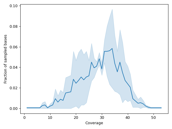
- plot_distribution(mode='aggregated', frac=0.1, ax=None, figsize=None, **kwargs)[source]
Create a line plot visualizaing the distribution of per-base read depth.
- Parameters:
mode ({‘aggregated’, ‘individual’}, default: ‘aggregated’) – Determines how to display the lines:
‘aggregated’: Aggregate over repeated values to show the mean and 95% confidence interval.
‘individual’: Show data for individual samples.
frac (float, default: 0.1) – Fraction of data to be sampled (to speed up the process).
ax (matplotlib.axes.Axes, optional) – Pre-existing axes for the plot. Otherwise, crete a new one.
figsize (tuple, optional) – Width, height in inches. Format: (float, float).
kwargs – Other keyword arguments will be passed down to
seaborn.lineplot().
- Returns:
The matplotlib axes containing the plot.
- Return type:
matplotlib.axes.Axes
Examples
By default (
mode='aggregated'), the method will aggregate over repeated values:>>> import matplotlib.pyplot as plt >>> import numpy as np >>> from fuc import pycov >>> data = { ... 'Chromosome': ['chr1'] * 1000, ... 'Position': np.arange(1000, 2000), ... 'A': pycov.simulate(loc=35, scale=5), ... 'B': pycov.simulate(loc=25, scale=7), ... } >>> cf = pycov.CovFrame.from_dict(data) >>> cf.plot_distribution(mode='aggregated', frac=0.9) >>> plt.tight_layout()
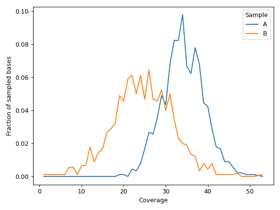
We can display data for individual samples:
>>> cf.plot_distribution(mode='individual', frac=0.9)
>>> plt.tight_layout()
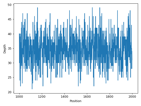
- plot_region(sample, region=None, samples=None, label=None, ax=None, figsize=None, **kwargs)[source]
Create read depth profile for specified region.
Region can be omitted if there is only one contig in the CovFrame.
- Parameters:
region (str, optional) – Target region (‘chrom:start-end’).
label (str, optional) – Label to use for the data points.
ax (matplotlib.axes.Axes, optional) – Pre-existing axes for the plot. Otherwise, crete a new one.
figsize (tuple, optional) – Width, height in inches. Format: (float, float).
kwargs – Other keyword arguments will be passed down to
seaborn.lineplot().
- Returns:
The matplotlib axes containing the plot.
- Return type:
matplotlib.axes.Axes
Examples
Below is a simple example:
>>> import matplotlib.pyplot as plt
>>> import numpy as np
>>> from fuc import pycov
>>> data = {
...    'Chromosome': ['chr1'] * 1000,
...    'Position': np.arange(1000, 2000),
...     'A': pycov.simulate(loc=35, scale=5),
...     'B': pycov.simulate(loc=25, scale=7),
... }
>>> cf = pycov.CovFrame.from_dict(data)
>>> ax = cf.plot_region('A')
>>> plt.tight_layout()
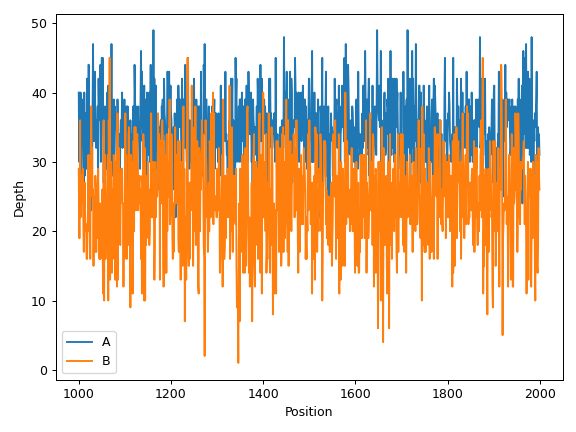
We can draw multiple profiles in one plot:
>>> ax = cf.plot_region('A', label='A')
>>> cf.plot_region('B', label='B', ax=ax)
>>> ax.legend()
>>> plt.tight_layout()
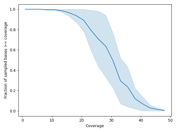
- plot_uniformity(mode='aggregated', frac=0.1, n=20, m=None, marker=None, ax=None, figsize=None, **kwargs)[source]
Create a line plot visualizing the uniformity in read depth.
- Parameters:
mode ({‘aggregated’, ‘individual’}, default: ‘aggregated’) – Determines how to display the lines:
‘aggregated’: Aggregate over repeated values to show the mean and 95% confidence interval.
‘individual’: Show data for individual samples.
frac (float, default: 0.1) – Fraction of data to be sampled (to speed up the process).
n (int or list, default: 20) – Number of evenly spaced points to generate for the x-axis. Alternatively, positions can be manually specified by providing a list.
m (float, optional) – Maximum point in the x-axis. By default, it will be the maximum depth in the entire dataset.
marker (str, optional) – Marker style string (e.g. ‘o’).
ax (matplotlib.axes.Axes, optional) – Pre-existing axes for the plot. Otherwise, crete a new one.
figsize (tuple, optional) – Width, height in inches. Format: (float, float).
kwargs – Other keyword arguments will be passed down to
seaborn.lineplot().
- Returns:
The matplotlib axes containing the plot.
- Return type:
matplotlib.axes.Axes
Examples
By default (
mode='aggregated'), the method will aggregate over repeated values:>>> import matplotlib.pyplot as plt >>> import numpy as np >>> from fuc import pycov >>> data = { ... 'Chromosome': ['chr1'] * 1000, ... 'Position': np.arange(1000, 2000), ... 'A': pycov.simulate(loc=35, scale=5), ... 'B': pycov.simulate(loc=25, scale=7), ... } >>> cf = pycov.CovFrame.from_dict(data) >>> cf.plot_uniformity(mode='aggregated') >>> plt.tight_layout()
We can display data for individual samples:
>>> cf.plot_uniformity(mode='individual')
>>> plt.tight_layout()
- rename(names, indicies=None)[source]
Rename the samples.
- Parameters:
names (dict or list) – Dict of old names to new names or list of new names.
indicies (list or tuple, optional) – List of 0-based sample indicies. Alternatively, a tuple (int, int) can be used to specify an index range.
- Returns:
Updated CovFrame.
- Return type:
Examples
>>> import numpy as np
>>> from fuc import pycov
>>> data = {
...     'Chromosome': ['chr1'] * 2,
...     'Position': np.arange(1, 3),
...     'A': pycov.simulate(loc=35, scale=5, size=2),
...     'B': pycov.simulate(loc=25, scale=7, size=2),
...     'C': pycov.simulate(loc=25, scale=7, size=2),
...     'D': pycov.simulate(loc=25, scale=7, size=2),
... }
>>> cf = pycov.CovFrame.from_dict(data)
>>> cf.df
  Chromosome  Position   A   B   C   D
0       chr1         1  31  19  28  15
1       chr1         2  35  24  22  17
>>> cf.rename(['1', '2', '3', '4']).df
  Chromosome  Position   1   2   3   4
0       chr1         1  31  19  28  15
1       chr1         2  35  24  22  17
>>> cf.rename({'B': '2', 'C': '3'}).df
  Chromosome  Position   A   2   3   D
0       chr1         1  31  19  28  15
1       chr1         2  35  24  22  17
>>> cf.rename(['2', '4'], indicies=[1, 3]).df
  Chromosome  Position   A   2   C   4
0       chr1         1  31  19  28  15
1       chr1         2  35  24  22  17
>>> cf.rename(['2', '3'], indicies=(1, 3)).df
  Chromosome  Position   A   2   3   D
0       chr1         1  31  19  28  15
1       chr1         2  35  24  22  17
- property samples
List of the sample names.
- Type:
list
- property shape
Dimensionality of CovFrame (positions, samples).
- Type:
tuple
- slice(region)[source]
Slice the CovFrame for the region.
- Parameters:
region (str) – Region (‘chrom:start-end’).
- Returns:
Sliced CovFrame.
- Return type:
Examples
>>> import numpy as np
>>> from fuc import pycov
>>> data = {
...     'Chromosome': ['chr1']*500 + ['chr2']*500,
...     'Position': np.arange(1000, 2000),
...     'A': pycov.simulate(loc=35, scale=5),
...     'B': pycov.simulate(loc=25, scale=7),
... }
>>> cf = pycov.CovFrame.from_dict(data)
>>> cf.slice('chr2').df.head()
  Chromosome  Position   A   B
0       chr2      1500  37  34
1       chr2      1501  28  12
2       chr2      1502  35  29
3       chr2      1503  34  34
4       chr2      1504  32  21
>>> cf.slice('chr2:1500-1504').df
  Chromosome  Position   A   B
0       chr2      1500  37  34
1       chr2      1501  28  12
2       chr2      1502  35  29
3       chr2      1503  34  34
4       chr2      1504  32  21
>>> cf.slice('chr2:-1504').df
  Chromosome  Position   A   B
0       chr2      1500  37  34
1       chr2      1501  28  12
2       chr2      1502  35  29
3       chr2      1503  34  34
4       chr2      1504  32  21
- subset(samples, exclude=False)[source]
Subset CovFrame for specified samples.
- Parameters:
samples (str or list) – Sample name or list of names (the order matters).
exclude (bool, default: False) – If True, exclude specified samples.
- Returns:
Subsetted CovFrame.
- Return type:
Examples
Assume we have the following data:
>>> import numpy as np
>>> from fuc import pycov
>>> data = {
...     'Chromosome': ['chr1'] * 1000,
...     'Position': np.arange(1000, 2000),
...     'A': pycov.simulate(loc=35, scale=5),
...     'B': pycov.simulate(loc=25, scale=7),
...     'C': pycov.simulate(loc=15, scale=2),
...     'D': pycov.simulate(loc=45, scale=8),
... }
>>> cf = pycov.CovFrame.from_dict(data)
>>> cf.df.head()
  Chromosome  Position   A   B   C   D
0       chr1      1000  30  30  15  37
1       chr1      1001  25  24  11  43
2       chr1      1002  33  24  16  50
3       chr1      1003  29  22  15  46
4       chr1      1004  34  30  11  32
We can subset the CovFrame for the samples A and B:
>>> cf.subset(['A', 'B']).df.head()
  Chromosome  Position   A   B
0       chr1      1000  30  30
1       chr1      1001  25  24
2       chr1      1002  33  24
3       chr1      1003  29  22
4       chr1      1004  34  30
Alternatively, we can exclude those samples:
>>> cf.subset(['A', 'B'], exclude=True).df.head()
  Chromosome  Position   C   D
0       chr1      1000  15  37
1       chr1      1001  11  43
2       chr1      1002  16  50
3       chr1      1003  15  46
4       chr1      1004  11  32
- to_file(fn, compression=False)[source]
Write the CovFrame to a TSV file.
If the file name ends with ‘.gz’, the method will automatically use the GZIP compression when writing the file.
- Parameters:
fn (str) – TSV file (compressed or uncompressed).
compression (bool, default: False) – If True, use the GZIP compression.
- to_string()[source]
Render the CovFrame to a console-friendly tabular output.
- Returns:
String representation of the CovFrame.
- Return type:
str
- update_chr_prefix(mode='remove')[source]
Add or remove the (annoying) ‘chr’ string from the Chromosome column.
- Parameters:
mode ({‘add’, ‘remove’}, default: ‘remove’) – Whether to add or remove the ‘chr’ string.
- Returns:
Updated CovFrame.
- Return type:
Examples
>>> import numpy as np
>>> from fuc import pycov
>>> data = {
...     'Chromosome': ['chr1'] * 3 + ['2'] * 3,
...     'Position': np.arange(1, 7),
...     'A': pycov.simulate(loc=35, scale=5, size=6),
...     'B': pycov.simulate(loc=25, scale=7, size=6),
... }
>>> cf = pycov.CovFrame.from_dict(data)
>>> cf.df
  Chromosome  Position   A   B
0       chr1         1  35  25
1       chr1         2  23  14
2       chr1         3  32  23
3          2         4  38  25
4          2         5  33   8
5          2         6  21  22
>>> cf.update_chr_prefix(mode='remove').df
  Chromosome  Position   A   B
0          1         1  35  25
1          1         2  23  14
2          1         3  32  23
3          2         4  38  25
4          2         5  33   8
5          2         6  21  22
>>> cf.update_chr_prefix(mode='add').df
  Chromosome  Position   A   B
0       chr1         1  35  25
1       chr1         2  23  14
2       chr1         3  32  23
3       chr2         4  38  25
4       chr2         5  33   8
5       chr2         6  21  22
- fuc.api.pycov.concat(cfs, axis=0)[source]
Concatenate CovFrame objects along a particular axis.
- Parameters:
cfs (list) – List of CovFrame objects.
axis ({0/’index’, 1/’columns’}, default: 0) – The axis to concatenate along.
- Returns:
Concatenated CovFrame.
- Return type:
- fuc.api.pycov.merge(cfs, how='inner')[source]
Merge CovFrame objects.
- Parameters:
cfs (list) – List of CovFrames to be merged. Note that the ‘chr’ prefix in contig names (e.g. ‘chr1’ vs. ‘1’) will be automatically added or removed as necessary to match the contig names of the first CovFrame.
how (str, default: ‘inner’) – Type of merge as defined in
pandas.merge().
- Returns:
Merged CovFrame.
- Return type:
See also
CovFrame.mergeMerge self with another CovFrame.
Examples
Assume we have the following data:
>>> import numpy as np
>>> from fuc import pycov
>>> data1 = {
...     'Chromosome': ['chr1'] * 5,
...     'Position': np.arange(100, 105),
...     'A': pycov.simulate(loc=35, scale=5, size=5),
...     'B': pycov.simulate(loc=25, scale=7, size=5),
... }
>>> data2 = {
...     'Chromosome': ['1'] * 5,
...     'Position': np.arange(102, 107),
...     'C': pycov.simulate(loc=35, scale=5, size=5),
... }
>>> cf1 = pycov.CovFrame.from_dict(data1)
>>> cf2 = pycov.CovFrame.from_dict(data2)
>>> cf1.df
  Chromosome  Position   A   B
0       chr1       100  33  17
1       chr1       101  36  20
2       chr1       102  39  39
3       chr1       103  31  19
4       chr1       104  31  10
>>> cf2.df
  Chromosome  Position   C
0          1       102  41
1          1       103  37
2          1       104  35
3          1       105  33
4          1       106  39
We can merge the two VcfFrames with how=’inner’ (default):
>>> pycov.merge([cf1, cf2]).df
  Chromosome  Position   A   B   C
0       chr1       102  39  39  41
1       chr1       103  31  19  37
2       chr1       104  31  10  35
We can also merge with how=’outer’:
>>> pycov.merge([cf1, cf2], how='outer').df
  Chromosome  Position     A     B     C
0       chr1       100  33.0  17.0   NaN
1       chr1       101  36.0  20.0   NaN
2       chr1       102  39.0  39.0  41.0
3       chr1       103  31.0  19.0  37.0
4       chr1       104  31.0  10.0  35.0
5       chr1       105   NaN   NaN  33.0
6       chr1       106   NaN   NaN  39.0
- fuc.api.pycov.simulate(mode='wgs', loc=30, scale=5, size=1000)[source]
Simulate read depth data for single sample.
Generated read depth will be integer and non-negative.
- Parameters:
mode ({‘wgs’}, default: ‘wgs’) – Additional modes will be made available in future releases.
loc (float, default: 30) – Mean (“centre”) of the distribution.
scale (float, default: 5) – Standard deviation (spread or “width”) of the distribution. Must be non-negative.
size (int, default: 1000) – Number of base pairs to return.
- Returns:
Numpy array object.
- Return type:
numpy.ndarray
Examples
>>> from fuc import pycov
>>> pycov.simulate(size=10)
array([25, 32, 30, 31, 26, 25, 33, 29, 28, 35])
fuc.pyfq
The pyfq submodule is designed for working with FASTQ files. It implements
pyfq.FqFrame which stores FASTQ data as pandas.DataFrame to allow
fast computation and easy manipulation.
Classes:
|
Class for storing FASTQ data. |
- class fuc.api.pyfq.FqFrame(df)[source]
Class for storing FASTQ data.
Methods:
from_file(fn)Construct FqFrame from a FASTQ file.
readlen()Return a dictionary of read lengths and their counts.
to_file(file_path)Write the FqFrame to a FASTQ file.
Attributes:
Number of sequence reads in the FqFrame.
- classmethod from_file(fn)[source]
Construct FqFrame from a FASTQ file.
- Parameters:
fn (str) – FASTQ file path (compressed or uncompressed).
- Returns:
FqFrame.
- Return type:
See also
FqFrameFqFrame object creation using constructor.
- property shape
Number of sequence reads in the FqFrame.
- Type:
int
fuc.pygff
The pygff submodule is designed for working with GFF/GTF files. It implements
pygff.GffFrame which stores GFF/GTF data as pandas.DataFrame to allow
fast computation and easy manipulation. The submodule strictly adheres to the
standard GFF specification.
A GFF/GTF file contains nine columns as follows:
No. |
Name |
Description |
Examples |
|---|---|---|---|
1 |
Seqid |
Landmark ID |
‘NC_000001.10’, ‘NC_012920.1’ |
2 |
Source |
Feature source |
‘RefSeq’, ‘BestRefSeq’, ‘Genescan’, ‘Genebank’ |
3 |
Type |
Feature type |
‘transcript’, ‘exon’, ‘gene’ |
4 |
Start |
Start coordinate |
11874, 14409 |
5 |
End |
End coordinate |
11874, 14409 |
6 |
Score |
Feature score |
‘.’, ‘1730.55’, ‘1070’ |
7 |
Strand |
Feature strand |
‘.’, ‘-’, ‘+’, ‘?’ |
8 |
Phase |
CDS phase |
‘.’, ‘0’, ‘1’, ‘2’ |
9 |
Attributes |
‘;’-separated attributes |
‘ID=NC_000001.10:1..249250621;Dbxref=taxon:9606;Name=1;chromosome=1;gbkey=Src;genome=chromosome;mol_type=genomic DNA’ |
Classes:
|
Class for storing GFF/GTF data. |
- class fuc.api.pygff.GffFrame(meta, df, fasta)[source]
Class for storing GFF/GTF data.
- Parameters:
meta (list) – List of metadata lines.
df (pandas.DataFrame) – DataFrame containing GFF/GTF data.
fasta (str) – FASTA sequence lines.
Attributes:
DataFrame containing GFF/GTF data.
FASTA sequence lines.
List of metadata lines.
Methods:
from_file(fn)Construct GffFrame from a GFF/GTF file.
protein_length(gene[, name])Return the protein length of a gene.
- property df
DataFrame containing GFF/GTF data.
- Type:
pandas.DataFrame
- property fasta
FASTA sequence lines.
- Type:
dict
- classmethod from_file(fn)[source]
Construct GffFrame from a GFF/GTF file.
- Parameters:
fn (str) – GFF/GTF file (compressed or uncompressed).
- Returns:
GffFrame object.
- Return type:
- property meta
List of metadata lines.
- Type:
list
fuc.pykallisto
The pykallisto submodule is designed for working with RNAseq quantification
data from Kallisto. It implements pykallisto.KallistoFrame which stores
Kallisto’s output data as pandas.DataFrame to allow fast computation and
easy manipulation. The pykallisto.KallistoFrame class also contains many
useful plotting methods such as KallistoFrame.plot_differential_abundance.
Classes:
|
Class for working with RNAseq quantification data from Kallisto. |
Functions:
|
A basic filter to be used. |
- class fuc.api.pykallisto.KallistoFrame(metadata, tx2gene, aggregation_column, filter_func=None, filter_target_id=None, filter_off=False)[source]
Class for working with RNAseq quantification data from Kallisto.
- Parameters:
metadata (pandas.DataFrame) – List of metadata lines.
tx2gene (pandas.DataFrame) – DataFrame containing transcript to gene mapping data.
aggregation_column (str) – Column name in
tx2geneto aggregate transcripts to the gene level.filter_func (func, optional) – Filtering function to be applied to each row (i.e. transcript). By default, the
pykallisto.basic_filter()method will be used.filter_target_id (list, optional) – Transcripts to filter using methods that can’t be implemented using
filter_func. If provided, this will overridefilter_func.filter_off (bool, default: False) – If True, do not apply any filtering. Useful for generating a simple count or tpm matrix.
Methods:
aggregate([filter])Aggregate transcript-level data to obtain gene-level data.
compute_fold_change(group, genes[, unit, flip])Compute fold change of gene expression between two groups.
plot_differential_abundance(gene, group[, ...])Plot differential abundance results for single gene.
- aggregate(filter=True)[source]
Aggregate transcript-level data to obtain gene-level data.
Running this method will set the attributes
KallistoFrame.df_gene_countandKallistoFrame.df_gene_tpm.- Parameters:
filter (bool, default: True) – If true, use filtered transcripts only. Otherwise, use all.
- compute_fold_change(group, genes, unit='tpm', flip=False)[source]
Compute fold change of gene expression between two groups.
- Parameters:
group (str) – Column in
KallistoFrame.metadataspecifying group information.gene (list) – Genes to compare.
unit ({‘tpm’, ‘count’}, default: ‘tpm’) – Abundance unit to display.
flip (bool, default: False) – If true, flip the denominator and numerator.
- plot_differential_abundance(gene, group, aggregate=True, filter=True, name='target_id', unit='tpm', ax=None, figsize=None)[source]
Plot differential abundance results for single gene.
- Parameters:
gene (str) – Gene to compare.
group (str) – Column in
KallistoFrame.metadataspecifying group information.aggregate (bool, default: True) – If true, display gene-level data (the
KallistoFrame.aggregate()method must be run beforehand). Otherwise, display transcript-level data.filter (bool, default: True) – If true, use filtered transcripts only. Otherwise, use all. Ignored when
aggregate=True.name (str, default: ‘target_id’) – Column in
KallistoFrame.tx2genespecifying transcript name to be displayed in the legend. Ignored whenaggregate=True.unit ({‘tpm’, ‘count’}, default: ‘tpm’) – Abundance unit to display.
ax (matplotlib.axes.Axes, optional) – Pre-existing axes for the plot. Otherwise, crete a new one.
figsize (tuple, optional) – Width, height in inches. Format: (float, float).
- Returns:
The matplotlib axes containing the plot.
- Return type:
matplotlib.axes.Axes
- fuc.api.pykallisto.basic_filter(row, min_reads=5, min_prop=0.47)[source]
A basic filter to be used.
By default, the method will filter out rows (i.e. transcripts) that do not have at least 5 estimated counts in at least 47% of the samples. Note that this is equivalent to the
sleuth.basic_filter()method.- Parameters:
row (pandas.Series) – This is a vector of numerics that will be passed in.
min_reads (int, default: 5) – The minimum number of estimated counts.
min_prop (float, default: 0.47) – The minimum proportion of samples.
- Returns:
A pandas series of boolean.
- Return type:
pd.Series
fuc.pymaf
The pymaf submodule is designed for working with MAF files. It implements
pymaf.MafFrame which stores MAF data as pandas.DataFrame to allow
fast computation and easy manipulation. The pymaf.MafFrame class also
contains many useful plotting methods such as MafFrame.plot_oncoplot and
MafFrame.plot_summary. The submodule strictly adheres to the
standard MAF specification.
A typical MAF file contains many columns ranging from gene symbol to protein change. However, most of the analysis in pymaf uses the following columns:
No. |
Name |
Description |
Examples |
|---|---|---|---|
1 |
Hugo_Symbol |
HUGO gene symbol |
‘TP53’, ‘Unknown’ |
2 |
Chromosome |
Chromosome name |
‘chr1’, ‘1’, ‘X’ |
3 |
Start_Position |
Start coordinate |
119031351 |
4 |
End_Position |
End coordinate |
44079555 |
5 |
Variant_Classification |
Translational effect |
‘Missense_Mutation’, ‘Silent’ |
6 |
Variant_Type |
Mutation type |
‘SNP’, ‘INS’, ‘DEL’ |
7 |
Reference_Allele |
Reference allele |
‘T’, ‘-’, ‘ACAA’ |
8 |
Tumor_Seq_Allele1 |
First tumor allele |
‘A’, ‘-’, ‘TCA’ |
9 |
Tumor_Seq_Allele2 |
Second tumor allele |
‘A’, ‘-’, ‘TCA’ |
10 |
Tumor_Sample_Barcode |
Sample ID |
‘TCGA-AB-3002’ |
11 |
Protein_Change |
Protein change |
‘p.L558Q’ |
It is also recommended to include additional custom columns such as variant allele frequecy (VAF) and transcript name.
If sample annotation data are available for a given MAF file, use
the common.AnnFrame class to import the data.
There are nine nonsynonymous variant classifcations that pymaf primarily uses: Missense_Mutation, Frame_Shift_Del, Frame_Shift_Ins, In_Frame_Del, In_Frame_Ins, Nonsense_Mutation, Nonstop_Mutation, Splice_Site, and Translation_Start_Site.
Classes:
|
Class for storing MAF data. |
- class fuc.api.pymaf.MafFrame(df)[source]
Class for storing MAF data.
- Parameters:
df (pandas.DataFrame) – DataFrame containing MAF data.
See also
MafFrame.from_fileConstruct MafFrame from a MAF file.
Methods:
calculate_concordance(a, b[, c, mode])Calculate genotype concordance between two (A, B) or three (A, B, C) samples.
compute_clonality(vaf_col[, threshold])Compute the clonality of variants based on VAF.
copy()Return a copy of the MafFrame.
filter_annot(af, expr)Filter the MafFrame using sample annotation data.
filter_indel([opposite, as_index])Remove rows with an indel.
from_file(fn)Construct MafFrame from a MAF file.
from_vcf(vcf[, keys, names])Construct MafFrame from a VCF file or VcfFrame.
get_gene_concordance(gene, a, b)Test whether two samples have the identical mutation profile for specified gene.
matrix_genes([mode, count])Compute a matrix of counts with a shape of (genes, variant classifications).
Compute a matrix of variant counts with a shape of (genes, samples).
Compute a matrix of variant counts with a shape of (samples, variant classifications).
matrix_waterfall([count, keep_empty])Compute a matrix of variant classifications with a shape of (genes, samples).
matrix_waterfall_matched(af, patient_col, ...)Compute a matrix of variant classifications with a shape of (gene-group pairs, patients).
plot_clonality(vaf_col[, af, group_col, ...])Create a bar plot summarizing the clonality of variants in top mutated genes.
plot_comparison(a, b[, c, labels, ax, figsize])Create a Venn diagram showing genotype concordance between groups.
plot_evolution(samples, vaf_col[, anchor, ...])Create a line plot visualizing changes in VAF between specified samples.
plot_genepair(x, y, vaf_col[, af, ...])Create a scatter plot of VAF between Gene X and Gene Y.
plot_genes([mode, count, flip, ax, figsize])Create a bar plot showing variant distirbution for top mutated genes.
plot_interactions([count, cmap, ax, figsize])Create a heatmap representing mutually exclusive or co-occurring set of genes.
plot_lollipop(gene[, alpha, ax, figsize, legend])Create a lollipop or stem plot showing amino acid changes of a gene.
plot_matrixg(gene, af, group_col[, ...])Create a heatmap of count matrix with a shape of (sample groups, protein changes).
plot_matrixs(gene[, samples, c0, c1, l0, ...])Create a heatmap of presence/absence matrix with a shape of (samples, protein changes).
plot_mutated([af, group_col, group_order, ...])Create a bar plot visualizing the mutation prevalence of top mutated genes.
plot_mutated_matched(af, patient_col, ...[, ...])Create a bar plot visualizing the mutation prevalence of top mutated genes.
plot_oncoplot([count, keep_empty, figsize, ...])Create an oncoplot.
plot_oncoplot_matched(af, patient_col, ...)Create an oncoplot for mached samples.
plot_rainfall(sample[, palette, legend, ax, ...])Create a rainfall plot visualizing inter-variant distance on a linear genomic scale for single sample.
plot_regplot_gene(af, group_col, a, b[, ...])Create a scatter plot with a linear regression model fit visualizing correlation between gene mutation frequencies in two sample groups A and B.
plot_regplot_tmb(af, subject_col, group_col, ...)Create a scatter plot with a linear regression model fit visualizing correlation between TMB in two sample groups.
plot_snvclsc([af, group_col, group_order, ...])Create a bar plot summarizing the count distrubtions of the six SNV classes for all samples.
plot_snvclsp([af, group_col, group_order, ...])Create a box plot summarizing the proportion distrubtions of the six SNV classes for all sample.
plot_snvclss([samples, color, colormap, ...])Create a bar plot showing the proportions of the six SNV classes for individual samples.
plot_summary([figsize, title_fontsize, ...])Create a summary figure for MafFrame.
plot_titv([af, group_col, group_order, ...])Create a box plot showing the Ti/Tv proportions of samples.
plot_tmb([samples, width, ax, figsize])Create a bar plot showing the TMB distributions of samples.
plot_tmb_matched(af, patient_col, group_col)Create a grouped bar plot showing TMB distributions for different group levels in each patient.
plot_vaf(vaf_col[, count, af, group_col, ...])Create a box plot showing the VAF distributions of top mutated genes.
plot_varcls([ax, figsize])Create a bar plot for the nonsynonymous variant classes.
plot_varsum([flip, ax, figsize])Create a summary box plot for variant classifications.
plot_vartype([palette, flip, ax, figsize])Create a bar plot summarizing the count distrubtions of viaration types for all samples.
plot_waterfall([count, keep_empty, samples, ...])Create a waterfall plot (oncoplot).
plot_waterfall_matched(af, patient_col, ...)Create a waterfall plot using matched samples from each patient.
subset(samples[, exclude])Subset MafFrame for specified samples.
to_file(fn)Write MafFrame to a MAF file.
Render MafFrame to a console-friendly tabular output.
to_vcf([fasta, ignore_indels, cols, names])Write the MafFrame to a sorted VcfFrame.
variants()List unique variants in MafFrame.
Attributes:
List of the genes.
List of the sample names.
Dimensionality of MafFrame (variants, samples).
- calculate_concordance(a, b, c=None, mode='all')[source]
Calculate genotype concordance between two (A, B) or three (A, B, C) samples.
This method will return (Ab, aB, AB, ab) for comparison between two samples and (Abc, aBc, ABc, abC, AbC, aBC, ABC, abc) for three samples. Note that the former is equivalent to (FP, FN, TP, TN) if we assume A is the test sample and B is the truth sample.
- Parameters:
a, b (str or int) – Name or index of Samples A and B.
c (str or int, optional) – Name or index of Sample C.
mode ({‘all’, ‘snv’, ‘indel’}, default: ‘all’) – Determines which variant types should be analyzed:
‘all’: Include both SNVs and INDELs.
‘snv’: Include SNVs only.
‘indel’: Include INDELs only.
- Returns:
Four- or eight-element tuple depending on the number of samples.
- Return type:
tuple
See also
fuc.api.common.sumstatReturn various summary statistics from (FP, FN, TP, TN).
Examples
>>> from fuc import common, pymaf
>>> common.load_dataset('tcga-laml')
>>> maf_file = '~/fuc-data/tcga-laml/tcga_laml.maf.gz'
>>> mf = pymaf.MafFrame.from_file(maf_file)
>>> mf.calculate_concordance('TCGA-AB-2988', 'TCGA-AB-2869')
(15, 12, 0, 2064)
>>> mf.calculate_concordance('TCGA-AB-2988', 'TCGA-AB-2869', 'TCGA-AB-3009')
(15, 12, 0, 42, 0, 0, 0, 2022)
- compute_clonality(vaf_col, threshold=0.25)[source]
Compute the clonality of variants based on VAF.
A mutation will be defined as “Subclonal” if the VAF is less than the threshold percentage (e.g. 25%) of the highest VAF in the sample and is defined as “Clonal” if it is equal to or above this threshold.
- Parameters:
vaf_col (str) – MafFrame column containing VAF data.
threshold (float) – Minimum VAF to be considered as “Clonal”.
- Returns:
Clonality for each variant.
- Return type:
panda.Series
Examples
>>> import matplotlib.pyplot as plt
>>> from fuc import common, pymaf
>>> common.load_dataset('tcga-laml')
>>> maf_file = '~/fuc-data/tcga-laml/tcga_laml.maf.gz'
>>> mf = pymaf.MafFrame.from_file(maf_file)
>>> mf.df['Clonality'] = mf.compute_clonality('i_TumorVAF_WU')
>>> mf.df['Clonality'][:10]
0    Clonal
1    Clonal
2    Clonal
3    Clonal
4    Clonal
5    Clonal
6    Clonal
7    Clonal
8    Clonal
9    Clonal
Name: Clonality, dtype: object
- filter_annot(af, expr)[source]
Filter the MafFrame using sample annotation data.
Samples are selected by querying the columns of an AnnFrame with a boolean expression. Samples not present in the MafFrame will be excluded automatically.
- Parameters:
af (AnnFrame) – AnnFrame containing sample annotation data.
expr (str) – Query expression to evaluate.
- Returns:
Filtered MafFrame.
- Return type:
Examples
>>> from fuc import common, pymaf
>>> common.load_dataset('tcga-laml')
>>> mf = pymaf.MafFrame.from_file('~/fuc-data/tcga-laml/tcga_laml.maf.gz')
>>> af = common.AnnFrame.from_file('~/fuc-data/tcga-laml/tcga_laml_annot.tsv', sample_col=0)
>>> filtered_mf = mf.filter_annot(af, "FAB_classification == 'M4'")
- filter_indel(opposite=False, as_index=False)[source]
Remove rows with an indel.
- Parameters:
opposite (bool, default: False) – If True, return rows that don’t meet the said criteria.
as_index (bool, default: False) – If True, return boolean index array instead of MafFrame.
- Returns:
Filtered MafFrame or boolean index array.
- Return type:
MafFrame or pandas.Series
Examples
>>> from fuc import common, pymaf
>>> common.load_dataset('tcga-laml')
>>> maf_file = '~/fuc-data/tcga-laml/tcga_laml.maf.gz'
>>> mf = pymaf.MafFrame.from_file(maf_file)
>>> mf.filter_indel().df.Variant_Type.unique()
array(['SNP'], dtype=object)
>>> mf.filter_indel(opposite=True).df.Variant_Type.unique()
array(['DEL', 'INS'], dtype=object)
- classmethod from_file(fn)[source]
Construct MafFrame from a MAF file.
- Parameters:
fn (str) – MAF file (compressed or uncompressed).
- Returns:
MafFrame object.
- Return type:
See also
MafFrameMafFrame object creation using constructor.
Examples
>>> from fuc import common, pymaf
>>> common.load_dataset('tcga-laml')
>>> maf_file = '~/fuc-data/tcga-laml/tcga_laml.maf.gz'
>>> mf = pymaf.MafFrame.from_file(maf_file)
- classmethod from_vcf(vcf, keys=None, names=None)[source]
Construct MafFrame from a VCF file or VcfFrame.
It is recommended that the input VCF data be functionally annotated by an annotation tool such as Ensembl VEP, SnpEff, and ANNOVAR; however, the method can handle unannotated VCF data as well.
The preferred tool for functional annotation is Ensembl VEP with “RefSeq transcripts” as the transcript database and the filtering option “Show one selected consequence per variant”.
- Parameters:
vcf (str or VcfFrame) – VCF file or VcfFrame.
keys (str or list) – Genotype key (e.g. ‘AD’, ‘AF’) or list of genotype keys to be added to the MafFrame.
names (str or list) – Column name or list of column names for
keys(must be the same length). By default, the genotype keys will be used as column names.
Examples
Below is a simple example:
>>> from fuc import pyvcf, pymaf
>>> data = {
...     'CHROM': ['chr1', 'chr2'],
...     'POS': [100, 101],
...     'ID': ['.', '.'],
...     'REF': ['G', 'T'],
...     'ALT': ['A', 'C'],
...     'QUAL': ['.', '.'],
...     'FILTER': ['.', '.'],
...     'INFO': ['CSQ=T|missense_variant|MODERATE|MTOR|2475|Transcript|NM_001386500.1|protein_coding|47/58||||6792|6644|2215|S/Y|tCt/tAt|rs587777894&COSV63868278&COSV63868313||-1||EntrezGene||||||||G|G||deleterious(0)|possibly_damaging(0.876)||||||||||||||||||likely_pathogenic&pathogenic|0&1&1|1&1&1|26619011&27159400&24631838&26018084&27830187|||||', 'CSQ=C|splice_donor_variant|HIGH|MTOR|2475|Transcript|NM_001386500.1|protein_coding||46/57||||||||||-1||EntrezGene||||||||A|A|||||||||||||||||||||||||||||'],
...     'FORMAT': ['GT:AD:DP:AF', 'GT:AD:DP:AF'],
...     'A': ['0/1:176,37:213:0.174', '0/1:966,98:1064:0.092']
... }
>>> vf = pyvcf.VcfFrame.from_dict([], data)
>>> vf.df
  CHROM  POS ID REF ALT QUAL FILTER                                               INFO       FORMAT                      A
0  chr1  100  .   G   A    .      .  CSQ=T|missense_variant|MODERATE|MTOR|2475|Tran...  GT:AD:DP:AF   0/1:176,37:213:0.174
1  chr2  101  .   T   C    .      .  CSQ=C|splice_donor_variant|HIGH|MTOR|2475|Tran...  GT:AD:DP:AF  0/1:966,98:1064:0.092
>>> mf = pymaf.MafFrame.from_vcf(vf)
>>> mf.df
  Hugo_Symbol Entrez_Gene_Id Center NCBI_Build Chromosome  Start_Position  End_Position Strand Variant_Classification Variant_Type Reference_Allele Tumor_Seq_Allele1 Tumor_Seq_Allele2 Protein_Change Tumor_Sample_Barcode
0        MTOR           2475      .          .       chr1             100           100      -      Missense_Mutation          SNP                G                 A                 A       p.S2215Y                    A
1        MTOR           2475      .          .       chr2             101           101      -            Splice_Site          SNP                T                 C                 C              .                    A
We can add genotype keys such as AD and AF:
>>> mf = pymaf.MafFrame.from_vcf(vf, keys=['AD', 'AF'])
>>> mf.df
  Hugo_Symbol Entrez_Gene_Id Center NCBI_Build Chromosome  Start_Position  End_Position Strand Variant_Classification Variant_Type Reference_Allele Tumor_Seq_Allele1 Tumor_Seq_Allele2 Protein_Change Tumor_Sample_Barcode      AD     AF
0        MTOR           2475      .          .       chr1             100           100      -      Missense_Mutation          SNP                G                 A                 A       p.S2215Y                    A  176,37  0.174
1        MTOR           2475      .          .       chr2             101           101      -            Splice_Site          SNP                T                 C                 C              .                    A  966,98  0.092
The method can accept a VCF file as input instead of VcfFrame:
>>> mf = pymaf.MafFrame.from_vcf('annotated.vcf')
The method can also handle unannotated VCF data:
>>> data = {
...     'CHROM': ['chr1', 'chr1', 'chr1'],
...     'POS': [100, 200, 300],
...     'ID': ['.', '.', '.'],
...     'REF': ['G', 'C', 'TTC'],
...     'ALT': ['A', 'CAG', 'T'],
...     'QUAL': ['.', '.', '.'],
...     'FILTER': ['.', '.', '.'],
...     'INFO': ['.', '.', '.'],
...     'FORMAT': ['GT', 'GT', 'GT'],
...     'A': ['0/1', '0/1', '0/1']
... }
>>> vf = pyvcf.VcfFrame.from_dict([], data)
>>> vf.df
  CHROM  POS ID  REF  ALT QUAL FILTER INFO FORMAT    A
0  chr1  100  .    G    A    .      .    .     GT  0/1
1  chr1  200  .    C  CAG    .      .    .     GT  0/1
2  chr1  300  .  TTC    T    .      .    .     GT  0/1
>>> mf = pymaf.MafFrame.from_vcf(vf)
>>> mf.df
  Hugo_Symbol Entrez_Gene_Id Center NCBI_Build Chromosome  Start_Position  End_Position Strand Variant_Classification Variant_Type Reference_Allele Tumor_Seq_Allele1 Tumor_Seq_Allele2 Protein_Change Tumor_Sample_Barcode
0           .              .      .          .       chr1             100           100      .                      .          SNP                G                 A                 A              .                    A
1           .              .      .          .       chr1             200           201      .                      .          INS                -                AG                AG              .                    A
2           .              .      .          .       chr1             301           302      .                      .          DEL               TC                 -                 -              .                    A
- property genes
List of the genes.
- Type:
list
- get_gene_concordance(gene, a, b)[source]
Test whether two samples have the identical mutation profile for specified gene.
- Parameters:
gene (str) – Name of the gene.
a, b (str) – Sample name.
- Returns:
True if the two samples have the same mutation profile.
- Return type:
bool
- matrix_genes(mode='variants', count=10)[source]
Compute a matrix of counts with a shape of (genes, variant classifications).
This method only considers the nine nonsynonymous variant classifications.
- Parameters:
mode ({‘variants’, ‘samples’}, default: ‘variants’) – Determines how to identify top mutated genes:
‘variants’: Count the number of observed variants.
‘samples’: Count the number of affected samples. Using this option will create an additional variant classification called ‘Multi_Hit’.
count (int, default: 10) – Number of top mutated genes to include.
- Returns:
The said matrix.
- Return type:
pandas.DataFrame
- matrix_prevalence()[source]
Compute a matrix of variant counts with a shape of (genes, samples).
- Returns:
The said matrix.
- Return type:
pandas.DataFrame
- matrix_tmb()[source]
Compute a matrix of variant counts with a shape of (samples, variant classifications).
- Returns:
The said matrix.
- Return type:
pandas.DataFrame
- matrix_waterfall(count=10, keep_empty=False)[source]
Compute a matrix of variant classifications with a shape of (genes, samples).
If there are multiple variant classifications available for a given cell, they will be replaced as ‘Multi_Hit’.
- Parameters:
count (int, default: 10) – Number of top mutated genes to include.
keep_empty (bool, default: False) – If True, keep samples with all
NaN’s.
- Returns:
The said matrix.
- Return type:
pandas.DataFrame
- matrix_waterfall_matched(af, patient_col, group_col, group_order, count=10)[source]
Compute a matrix of variant classifications with a shape of (gene-group pairs, patients).
- Parameters:
af (AnnFrame) – AnnFrame containing sample annotation data.
patient_col (str) – AnnFrame column containing patient information.
group_col (str) – AnnFrame column containing sample group information.
group_order (list) – List of sample group names.
count (int, default: 10) – Number of top mutated genes to include.
ax (matplotlib.axes.Axes, optional) – Pre-existing axes for the plot. Otherwise, crete a new one.
figsize (tuple, optional) – Width, height in inches. Format: (float, float).
- Returns:
The matplotlib axes containing the plot.
- Return type:
matplotlib.axes.Axes
- plot_clonality(vaf_col, af=None, group_col=None, group_order=None, count=10, threshold=0.25, subclonal=False, ax=None, figsize=None)[source]
Create a bar plot summarizing the clonality of variants in top mutated genes.
Clonality will be calculated based on VAF using
MafFrame.compute_clonality().- Parameters:
vaf_col (str) – MafFrame column containing VAF data.
af (AnnFrame, optional) – AnnFrame containing sample annotation data.
group_col (str, optional) – AnnFrame column containing sample group information.
group_order (list, optional) – List of sample group names.
count (int, defualt: 10) – Number of top mutated genes to display.
threshold (float, default: 0.25) – VAF threshold percentage.
subclonal (bool, default: False) – If True, display subclonality (1 - clonality).
ax (matplotlib.axes.Axes, optional) – Pre-existing axes for the plot. Otherwise, crete a new one.
figsize (tuple, optional) – Width, height in inches. Format: (float, float).
kwargs – Other keyword arguments will be passed down to
seaborn.barplot().
- Returns:
The matplotlib axes containing the plot.
- Return type:
matplotlib.axes.Axes
See also
MafFrame.compute_clonalityCompute the clonality of variants based on VAF.
Examples
Below is a simple example:
>>> import matplotlib.pyplot as plt
>>> from fuc import common, pymaf
>>> common.load_dataset('tcga-laml')
>>> maf_file = '~/fuc-data/tcga-laml/tcga_laml.maf.gz'
>>> mf = pymaf.MafFrame.from_file(maf_file)
>>> mf.plot_clonality('i_TumorVAF_WU')
>>> plt.tight_layout()
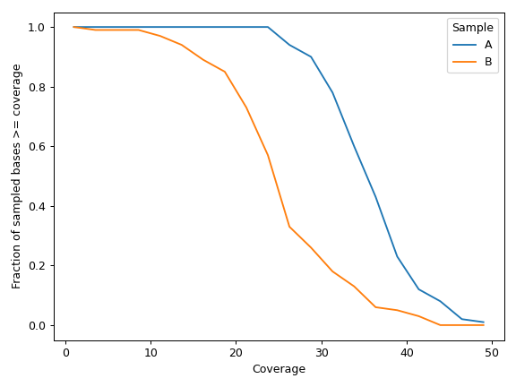
We can create a grouped bar plot based on FAB classification:
>>> annot_file = '~/fuc-data/tcga-laml/tcga_laml_annot.tsv'
>>> af = common.AnnFrame.from_file(annot_file, sample_col=0)
>>> mf.plot_clonality('i_TumorVAF_WU',
...                   af=af,
...                   group_col='FAB_classification',
...                   group_order=['M0', 'M1', 'M2'])
>>> plt.tight_layout()
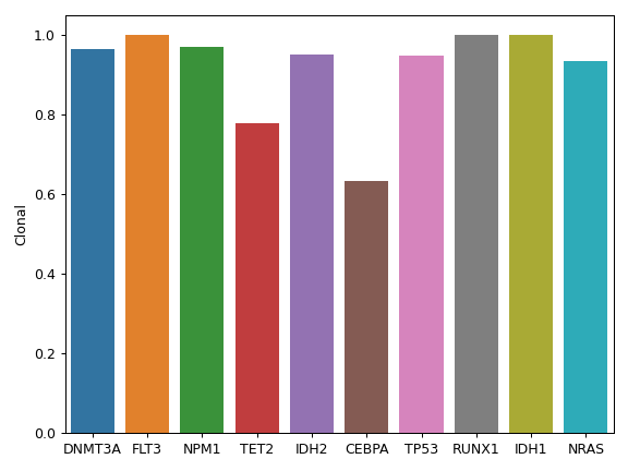
- plot_comparison(a, b, c=None, labels=None, ax=None, figsize=None)[source]
Create a Venn diagram showing genotype concordance between groups.
This method supports comparison between two groups (Groups A & B) as well as three groups (Groups A, B, & C).
- Parameters:
a, b (list) – Sample names. The lists must have the same shape.
c (list, optional) – Same as above.
labels (list, optional) – List of labels to be displayed.
ax (matplotlib.axes.Axes, optional) – Pre-existing axes for the plot. Otherwise, crete a new one.
figsize (tuple, optional) – Width, height in inches. Format: (float, float).
- Returns:
matplotlib.axes.Axes – The matplotlib axes containing the plot.
matplotlib_venn._common.VennDiagram – VennDiagram object.
- plot_evolution(samples, vaf_col, anchor=None, normalize=True, count=5, ax=None, figsize=None, **kwargs)[source]
Create a line plot visualizing changes in VAF between specified samples.
- Parameters:
samples (list) – List of samples to display.
vaf_col (str) – MafFrame column containing VAF data.
anchor (str, optional) – Sample to use as the anchor. If absent, use the first sample in the list.
normalize (bool, default: True) – If False, do not normalize VAF by the maximum value.
count (int, default: 5) – Number of top variants to display.
ax (matplotlib.axes.Axes, optional) – Pre-existing axes for the plot. Otherwise, crete a new one.
figsize (tuple, optional) – Width, height in inches. Format: (float, float).
kwargs – Other keyword arguments will be passed down to
seaborn.lineplot().
- Returns:
The matplotlib axes containing the plot.
- Return type:
matplotlib.axes.Axes
- plot_genepair(x, y, vaf_col, af=None, group_col=None, group_order=None, ax=None, figsize=None, **kwargs)[source]
Create a scatter plot of VAF between Gene X and Gene Y.
- Parameters:
x, y (str) – Gene names.
vaf_col (str) – MafFrame column containing VAF data.
af (AnnFrame, optional) – AnnFrame containing sample annotation data.
group_col (str, optional) – AnnFrame column containing sample group information.
group_order (list, optional) – List of sample group names.
ax (matplotlib.axes.Axes, optional) – Pre-existing axes for the plot. Otherwise, crete a new one.
figsize (tuple, optional) – Width, height in inches. Format: (float, float).
kwargs – Other keyword arguments will be passed down to
seaborn.scatterplot().
- Returns:
The matplotlib axes containing the plot.
- Return type:
matplotlib.axes.Axes
Examples
Below is a simple example:
>>> import matplotlib.pyplot as plt
>>> import seaborn as sns
>>> from fuc import common, pymaf
>>> common.load_dataset('tcga-laml')
>>> maf_file = '~/fuc-data/tcga-laml/tcga_laml.maf.gz'
>>> mf = pymaf.MafFrame.from_file(maf_file)
>>> mf.plot_genepair('DNMT3A', 'FLT3', 'i_TumorVAF_WU')
>>> plt.tight_layout()
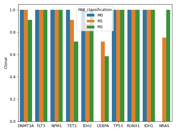
We can create a grouped bar plot based on FAB classification:
>>> annot_file = '~/fuc-data/tcga-laml/tcga_laml_annot.tsv'
>>> af = common.AnnFrame.from_file(annot_file, sample_col=0)
>>> mf.plot_genepair('DNMT3A', 'FLT3', 'i_TumorVAF_WU',
...                  af=af,
...                  group_col='FAB_classification')
>>> plt.tight_layout()
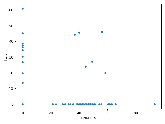
- plot_genes(mode='variants', count=10, flip=False, ax=None, figsize=None, **kwargs)[source]
Create a bar plot showing variant distirbution for top mutated genes.
- Parameters:
mode ({‘variants’, ‘samples’}, default: ‘variants’) – Determines how to identify top mutated genes:
‘variants’: Count the number of observed variants.
‘samples’: Count the number of affected samples. Using this option will create an additional variant classification called ‘Multi_Hit’.
count (int, default: 10) – Number of top mutated genes to display.
flip (bool, default: False) – If True, flip the x and y axes.
ax (matplotlib.axes.Axes, optional) – Pre-existing axes for the plot. Otherwise, crete a new one.
figsize (tuple, optional) – Width, height in inches. Format: (float, float).
kwargs – Other keyword arguments will be passed down to
pandas.DataFrame.plot.bar()orpandas.DataFrame.plot.barh().
- Returns:
The matplotlib axes containing the plot.
- Return type:
matplotlib.axes.Axes
Examples
By default (
mode='variants'), the method identifies top mutated genes by counting the number of observed variants:>>> import matplotlib.pyplot as plt >>> from fuc import common, pymaf >>> common.load_dataset('tcga-laml') >>> maf_file = '~/fuc-data/tcga-laml/tcga_laml.maf.gz' >>> mf = pymaf.MafFrame.from_file(maf_file) >>> mf.plot_genes() >>> plt.tight_layout()
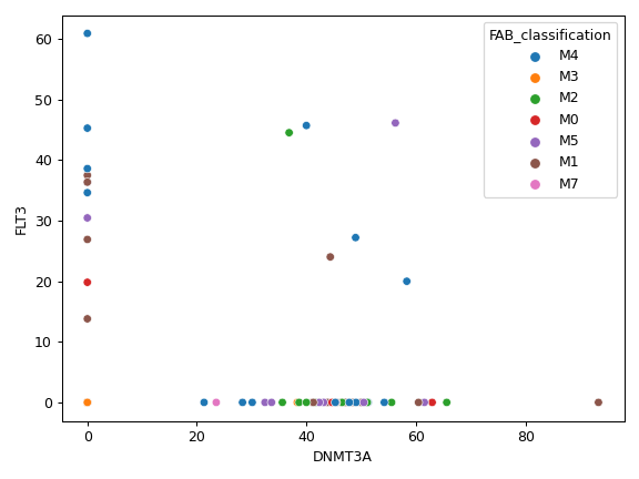
We can also identify top mutated genes by counting the number of affected samples:
>>> mf.plot_genes(mode='samples')
>>> plt.tight_layout()
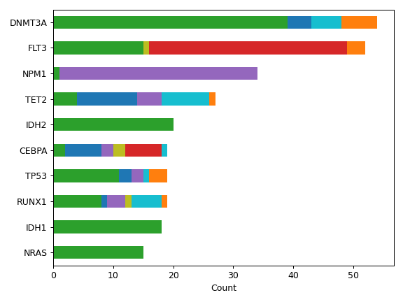
- plot_interactions(count=10, cmap=None, ax=None, figsize=None, **kwargs)[source]
Create a heatmap representing mutually exclusive or co-occurring set of genes.
This method performs pair-wise Fisher’s Exact test to detect such significant pair of genes.
- Parameters:
count (int, defualt: 10) – Number of top mutated genes to display.
cmap (str, optional) – Color map.
ax (matplotlib.axes.Axes, optional) – Pre-existing axes for the plot. Otherwise, crete a new one.
figsize (tuple, optional) – Width, height in inches. Format: (float, float).
kwargs – Other keyword arguments will be passed down to
seaborn.heatmap().
- Returns:
The matplotlib axes containing the plot.
- Return type:
matplotlib.axes.Axes
Examples
>>> import matplotlib.pyplot as plt
>>> from fuc import common, pymaf
>>> common.load_dataset('tcga-laml')
>>> maf_file = '~/fuc-data/tcga-laml/tcga_laml.maf.gz'
>>> mf = pymaf.MafFrame.from_file(maf_file)
>>> mf.plot_interactions(count=25, cmap='BrBG')
>>> plt.tight_layout()
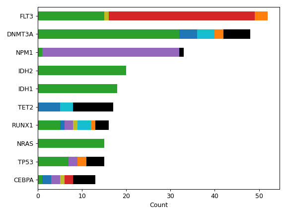
- plot_lollipop(gene, alpha=0.7, ax=None, figsize=None, legend=True)[source]
Create a lollipop or stem plot showing amino acid changes of a gene.
- Parameters:
gene (str) – Name of the gene.
alpha (float, default: 0.7) – Set the color transparency. Must be within the 0-1 range, inclusive.
ax (matplotlib.axes.Axes, optional) – Pre-existing axes for the plot. Otherwise, crete a new one.
figsize (tuple, optional) – Width, height in inches. Format: (float, float).
- Returns:
The matplotlib axes containing the plot.
- Return type:
matplotlib.axes.Axes
Examples
>>> import matplotlib.pyplot as plt
>>> from fuc import common, pymaf
>>> common.load_dataset('tcga-laml')
>>> maf_file = '~/fuc-data/tcga-laml/tcga_laml.maf.gz'
>>> mf = pymaf.MafFrame.from_file(maf_file)
>>> mf.plot_lollipop('DNMT3A')
>>> plt.tight_layout()
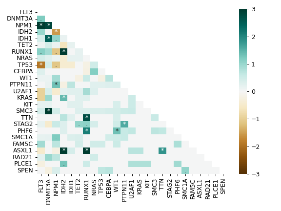
- plot_matrixg(gene, af, group_col, group_order=None, cbar=True, ax=None, figsize=None, **kwargs)[source]
Create a heatmap of count matrix with a shape of (sample groups, protein changes).
- Parameters:
gene (str) – Name of the gene.
af (AnnFrame) – AnnFrame containing sample annotation data.
group_col (str) – AnnFrame column containing sample group information.
group_order (list, optional) – List of sample group names.
cbar (bool, default: True) – Whether to draw a colorbar.
ax (matplotlib.axes.Axes, optional) – Pre-existing axes for the plot. Otherwise, crete a new one.
figsize (tuple, optional) – Width, height in inches. Format: (float, float).
kwargs – Other keyword arguments will be passed down to
seaborn.heatmap().
- Returns:
The matplotlib axes containing the plot.
- Return type:
matplotlib.axes.Axes
Examples
>>> import matplotlib.pyplot as plt
>>> from fuc import common, pymaf
>>> common.load_dataset('tcga-laml')
>>> maf_file = '~/fuc-data/tcga-laml/tcga_laml.maf.gz'
>>> annot_file = '~/fuc-data/tcga-laml/tcga_laml_annot.tsv'
>>> mf = pymaf.MafFrame.from_file(maf_file)
>>> af = common.AnnFrame.from_file(annot_file, sample_col=0)
>>> mf.plot_matrixg('IDH1', af, 'FAB_classification', linewidth=0.5, square=True, annot=True)
>>> plt.tight_layout()
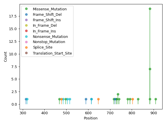
- plot_matrixs(gene, samples=None, c0='lightgray', c1='red', l0='0', l1='1', cbar=True, square=False, ax=None, figsize=None, **kwargs)[source]
Create a heatmap of presence/absence matrix with a shape of (samples, protein changes).
- Parameters:
gene (str) – Name of the gene.
samples (list, optional) – List of samples to display (in that order too). If samples that are absent in the MafFrame are provided, the method will give a warning but still draw an empty bar for those samples.
c0 (str, default: ‘lightgray’) – Color for absence.
c1 (str, default: ‘red’) – Color for presence.
l0 (str, default: ‘0’) – Label for absence.
l1 (str, default: ‘1’) – Label for presence.
cbar (bool, default: True) – Whether to draw a colorbar.
square (bool, default: False) – If True, set the Axes aspect to “equal” so each cell will be square-shaped.
ax (matplotlib.axes.Axes, optional) – Pre-existing axes for the plot. Otherwise, crete a new one.
figsize (tuple, optional) – Width, height in inches. Format: (float, float).
kwargs – Other keyword arguments will be passed down to
seaborn.heatmap().
- Returns:
The matplotlib axes containing the plot.
- Return type:
matplotlib.axes.Axes
Examples
>>> import matplotlib.pyplot as plt
>>> from fuc import common, pymaf
>>> common.load_dataset('tcga-laml')
>>> maf_file = '~/fuc-data/tcga-laml/tcga_laml.maf.gz'
>>> mf = pymaf.MafFrame.from_file(maf_file)
>>> mf.plot_matrixs('KRAS', linewidth=0.5, square=True)
>>> plt.tight_layout()
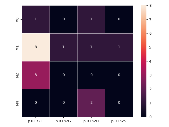
- plot_mutated(af=None, group_col=None, group_order=None, genes=None, count=10, ax=None, figsize=None)[source]
Create a bar plot visualizing the mutation prevalence of top mutated genes.
- Parameters:
af (AnnFrame, optional) – AnnFrame containing sample annotation data.
group_col (str, optional) – AnnFrame column containing sample group information.
group_order (list, optional) – List of sample group names.
genes (list, optional) – Genes to display. When absent, top mutated genes (
count) will be used.count (int, defualt: 10) – Number of top mutated genes to display. Ignored if
genesis specified.ax (matplotlib.axes.Axes, optional) – Pre-existing axes for the plot. Otherwise, crete a new one.
figsize (tuple, optional) – Width, height in inches. Format: (float, float).
kwargs – Other keyword arguments will be passed down to
seaborn.barplot().
- Returns:
The matplotlib axes containing the plot.
- Return type:
matplotlib.axes.Axes
Examples
Below is a simple example:
>>> import matplotlib.pyplot as plt
>>> import seaborn as sns
>>> from fuc import common, pymaf
>>> common.load_dataset('tcga-laml')
>>> maf_file = '~/fuc-data/tcga-laml/tcga_laml.maf.gz'
>>> mf = pymaf.MafFrame.from_file(maf_file)
>>> mf.plot_mutated()
>>> plt.tight_layout()
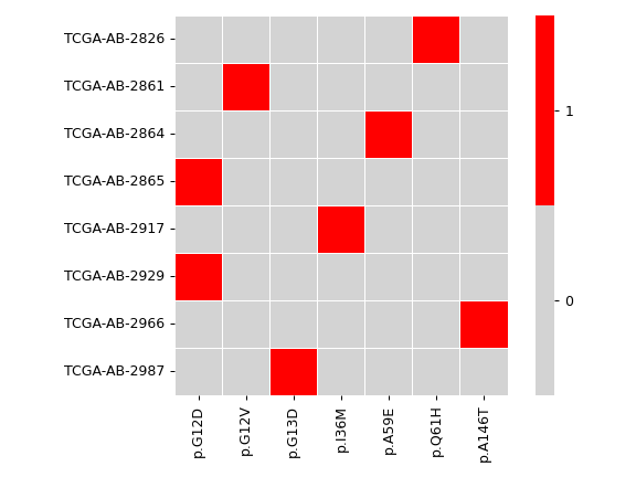
We can create a grouped bar plot based on FAB classification:
>>> annot_file = '~/fuc-data/tcga-laml/tcga_laml_annot.tsv'
>>> af = common.AnnFrame.from_file(annot_file, sample_col=0)
>>> mf.plot_mutated(af=af,
...                 group_col='FAB_classification',
...                 group_order=['M0', 'M1', 'M2'])
>>> plt.tight_layout()
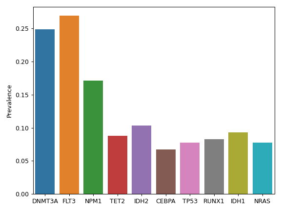
- plot_mutated_matched(af, patient_col, group_col, group_order, count=10, ax=None, figsize=None, **kwargs)[source]
Create a bar plot visualizing the mutation prevalence of top mutated genes.
- Parameters:
af (AnnFrame) – AnnFrame containing sample annotation data.
patient_col (str) – AnnFrame column containing patient information.
group_col (str) – AnnFrame column containing sample group information.
group_order (list) – List of sample group names.
count (int, defualt: 10) – Number of top mutated genes to display.
ax (matplotlib.axes.Axes, optional) – Pre-existing axes for the plot. Otherwise, crete a new one.
figsize (tuple, optional) – Width, height in inches. Format: (float, float).
kwargs – Other keyword arguments will be passed down to
seaborn.barplot().
- Returns:
The matplotlib axes containing the plot.
- Return type:
matplotlib.axes.Axes
- plot_oncoplot(count=10, keep_empty=False, figsize=(15, 10), label_fontsize=15, ticklabels_fontsize=15, legend_fontsize=15)[source]
Create an oncoplot.
See this tutorial to learn how to create customized oncoplots.
- Parameters:
count (int, default: 10) – Number of top mutated genes to display.
keep_empty (bool, default: False) – If True, display samples that do not have any mutations.
figsize (tuple, default: (15, 10)) – Width, height in inches. Format: (float, float).
label_fontsize (float, default: 15) – Font size of labels.
ticklabels_fontsize (float, default: 15) – Font size of tick labels.
legend_fontsize (float, default: 15) – Font size of legend texts.
Examples
>>> import matplotlib.pyplot as plt
>>> from fuc import common, pymaf
>>> common.load_dataset('tcga-laml')
>>> maf_file = '~/fuc-data/tcga-laml/tcga_laml.maf.gz'
>>> mf = pymaf.MafFrame.from_file(maf_file)
>>> mf.plot_oncoplot()
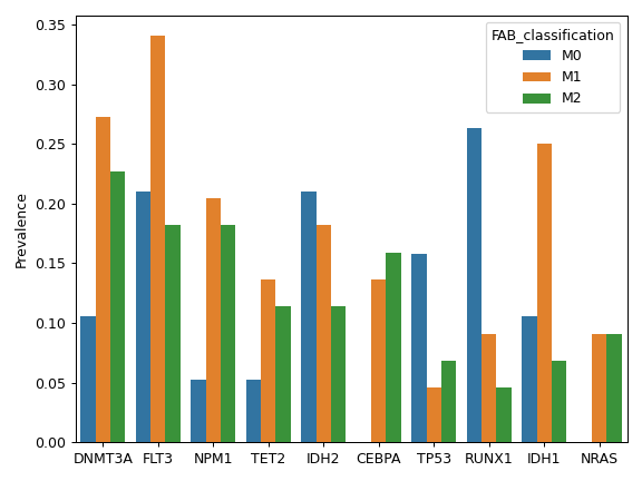
- plot_oncoplot_matched(af, patient_col, group_col, group_order, colors='Set2', figsize=(15, 10), label_fontsize=12, ticklabels_fontsize=12, legend_fontsize=12)[source]
Create an oncoplot for mached samples.
- Parameters:
af (AnnFrame) – AnnFrame containing sample annotation data.
patient_col (str) – AnnFrame column containing patient information.
group_col (str) – AnnFrame column containing sample group information.
group_order (list, optional) – List of sample group names.
colors (str) – Colormap name for the sample groups.
figsize (tuple, default: (15, 10)) – Width, height in inches. Format: (float, float).
label_fontsize (float, default: 12) – Font size of labels.
ticklabels_fontsize (float, default: 12) – Font size of tick labels.
legend_fontsize (float, default: 12) – Font size of legend texts.
- plot_rainfall(sample, palette=None, legend='auto', ax=None, figsize=None, **kwargs)[source]
Create a rainfall plot visualizing inter-variant distance on a linear genomic scale for single sample.
- Parameters:
sample (str) – Name of the sample.
palette (str, optional) – Name of the seaborn palette. See the Control plot colors tutorial for details.
legend ({‘auto’, ‘brief’, ‘full’, False}, default: ‘auto’) – Display setting of the legend according to
seaborn.scatterplot().ax (matplotlib.axes.Axes, optional) – Pre-existing axes for the plot. Otherwise, crete a new one.
figsize (tuple, optional) – Width, height in inches. Format: (float, float).
kwargs – Other keyword arguments will be passed down to
seaborn.scatterplot().
- Returns:
The matplotlib axes containing the plot.
- Return type:
matplotlib.axes.Axes
Examples
>>> import matplotlib.pyplot as plt
>>> import seaborn as sns
>>> from fuc import common, pymaf
>>> common.load_dataset('brca')
>>> maf_file = '~/fuc-data/brca/brca.maf.gz'
>>> mf = pymaf.MafFrame.from_file(maf_file)
>>> mf.plot_rainfall('TCGA-A8-A08B',
...                  figsize=(14, 7),
...                  palette=sns.color_palette('Set2')[:6])
>>> plt.tight_layout()
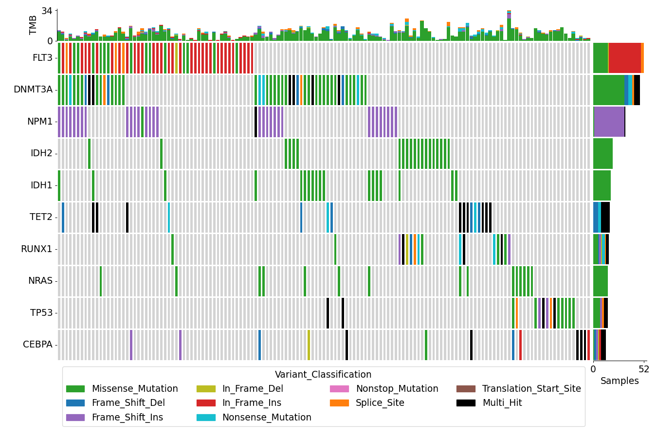
- plot_regplot_gene(af, group_col, a, b, a_size=None, b_size=None, genes=None, count=10, to_csv=None, ax=None, figsize=None, **kwargs)[source]
Create a scatter plot with a linear regression model fit visualizing correlation between gene mutation frequencies in two sample groups A and B.
Each point in the plot represents a gene.
The method will automatically calculate and print summary statistics including R-squared and p-value.
- Parameters:
af (AnnFrame) – AnnFrame containing sample annotation data.
group_col (str) – AnnFrame column containing sample group information.
a, b (str) – Sample group names.
a_size, b_size (int, optional) – Sample group sizes to use as denominator. By default, these are inferred from the MafFrame and AnnFrame objects.
genes (list, optional) – Genes to display. When absent, top mutated genes (
count) will be used.count (int, defualt: 10) – Number of top mutated genes to display. Ignored if
genesis specified.to_csv (str, optional) – Write the plot’s data to a CSV file.
ax (matplotlib.axes.Axes, optional) – Pre-existing axes for the plot. Otherwise, crete a new one.
figsize (tuple, optional) – Width, height in inches. Format: (float, float).
kwargs – Other keyword arguments will be passed down to
seaborn.regplot().
- Returns:
The matplotlib axes containing the plot.
- Return type:
matplotlib.axes.Axes
Examples
>>> import matplotlib.pyplot as plt
>>> from fuc import common, pymaf
>>> common.load_dataset('tcga-laml')
>>> maf_file = '~/fuc-data/tcga-laml/tcga_laml.maf.gz'
>>> annot_file = '~/fuc-data/tcga-laml/tcga_laml_annot.tsv'
>>> mf = pymaf.MafFrame.from_file(maf_file)
>>> af = common.AnnFrame.from_file(annot_file, sample_col=0)
>>> mf.plot_regplot_gene(af, 'FAB_classification', 'M1', 'M2')
Results for M2 ~ M1:
R^2 = 0.43
  P = 3.96e-02
>>> plt.tight_layout()

- plot_regplot_tmb(af, subject_col, group_col, a, b, ax=None, figsize=None, to_csv=None, **kwargs)[source]
Create a scatter plot with a linear regression model fit visualizing correlation between TMB in two sample groups.
The method will automatically calculate and print summary statistics including R-squared and p-value.
- Parameters:
af (AnnFrame) – AnnFrame containing sample annotation data.
subject_col (str) – AnnFrame column containing sample subject information.
group_col (str) – AnnFrame column containing sample group information.
a, b (str) – Sample group names.
to_csv (str, optional) – Write the plot’s data to a CSV file.
ax (matplotlib.axes.Axes, optional) – Pre-existing axes for the plot. Otherwise, crete a new one.
figsize (tuple, optional) – Width, height in inches. Format: (float, float).
kwargs – Other keyword arguments will be passed down to
seaborn.regplot().
- Returns:
The matplotlib axes containing the plot.
- Return type:
matplotlib.axes.Axes
See also
fuc.api.pyvcf.VcfFrame.plot_regplot_tmbSimilar method for the
fuc.api.pyvcf.VcfFrame()class.
Examples
>>> import matplotlib.pyplot as plt
>>> from fuc import common, pymaf, pyvcf
>>> common.load_dataset('pyvcf')
>>> vcf_file = '~/fuc-data/pyvcf/normal-tumor.vcf'
>>> annot_file = '~/fuc-data/pyvcf/normal-tumor-annot.tsv'
>>> vf = pyvcf.VcfFrame.from_file(vcf_file)
>>> af = common.AnnFrame.from_file(annot_file, sample_col='Sample')
>>> mf = pymaf.MafFrame.from_vcf(vf)
>>> mf.plot_regplot_tmb(af, 'Patient', 'Tissue', 'Normal', 'Tumor')
Results for Tumor ~ Normal:
R^2 = 0.01
  P = 7.17e-01
>>> plt.tight_layout()
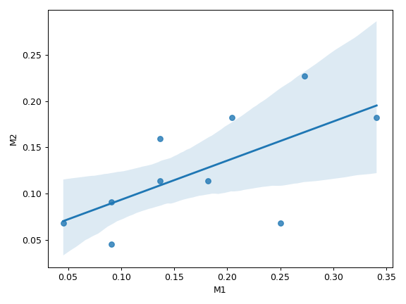
- plot_snvclsc(af=None, group_col=None, group_order=None, palette=None, flip=False, ax=None, figsize=None, **kwargs)[source]
Create a bar plot summarizing the count distrubtions of the six SNV classes for all samples.
A grouped bar plot can be created with
group_col(requires an AnnFrame).- Parameters:
af (AnnFrame, optional) – AnnFrame containing sample annotation data.
group_col (str, optional) – AnnFrame column containing sample group information.
group_order (list, optional) – List of sample group names.
palette (str, optional) – Name of the seaborn palette. See the Control plot colors tutorial for details.
flip (bool, default: False) – If True, flip the x and y axes.
ax (matplotlib.axes.Axes, optional) – Pre-existing axes for the plot. Otherwise, crete a new one.
figsize (tuple, optional) – Width, height in inches. Format: (float, float).
kwargs – Other keyword arguments will be passed down to
seaborn.barplot().
- Returns:
The matplotlib axes containing the plot.
- Return type:
matplotlib.axes.Axes
See also
MafFrame.plot_snvclspCreate a box plot summarizing the proportion distrubtions of the six SNV classes for all sample.
MafFrame.plot_snvclssCreate a bar plot showing the proportions of the six SNV classes for individual samples.
Examples
Below is a simple example:
>>> import matplotlib.pyplot as plt
>>> import seaborn as sns
>>> from fuc import common, pymaf
>>> common.load_dataset('tcga-laml')
>>> maf_file = '~/fuc-data/tcga-laml/tcga_laml.maf.gz'
>>> mf = pymaf.MafFrame.from_file(maf_file)
>>> mf.plot_snvclsc(palette=sns.color_palette('Dark2'))
>>> plt.tight_layout()
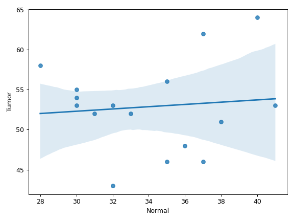
We can create a grouped bar plot based on FAB classification:
>>> annot_file = '~/fuc-data/tcga-laml/tcga_laml_annot.tsv'
>>> af = common.AnnFrame.from_file(annot_file, sample_col=0)
>>> mf.plot_snvclsc(af=af,
...                 group_col='FAB_classification',
...                 group_order=['M0', 'M1', 'M2'])
>>> plt.tight_layout()
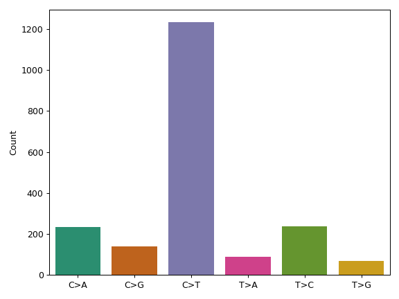
- plot_snvclsp(af=None, group_col=None, group_order=None, palette=None, flip=False, ax=None, figsize=None, **kwargs)[source]
Create a box plot summarizing the proportion distrubtions of the six SNV classes for all sample.
- Parameters:
af (AnnFrame, optional) – AnnFrame containing sample annotation data.
group_col (str, optional) – AnnFrame column containing sample group information.
group_order (list, optional) – List of sample group names.
palette (str, optional) – Name of the seaborn palette. See the Control plot colors tutorial for details.
flip (bool, default: False) – If True, flip the x and y axes.
ax (matplotlib.axes.Axes, optional) – Pre-existing axes for the plot. Otherwise, crete a new one.
figsize (tuple, optional) – Width, height in inches. Format: (float, float).
kwargs – Other keyword arguments will be passed down to
seaborn.boxplot().
- Returns:
The matplotlib axes containing the plot.
- Return type:
matplotlib.axes.Axes
See also
MafFrame.plot_snvclscCreate a bar plot summarizing the count distrubtions of the six SNV classes for all samples.
MafFrame.plot_snvclssCreate a bar plot showing the proportions of the six SNV classes for individual samples.
Examples
Below is a simple example:
>>> import matplotlib.pyplot as plt
>>> import seaborn as sns
>>> from fuc import common, pymaf
>>> common.load_dataset('tcga-laml')
>>> maf_file = '~/fuc-data/tcga-laml/tcga_laml.maf.gz'
>>> mf = pymaf.MafFrame.from_file(maf_file)
>>> mf.plot_snvclsp(palette=sns.color_palette('Set2'))
>>> plt.tight_layout()

We can create a grouped bar plot based on FAB classification:
>>> annot_file = '~/fuc-data/tcga-laml/tcga_laml_annot.tsv'
>>> af = common.AnnFrame.from_file(annot_file, sample_col=0)
>>> mf.plot_snvclsp(af=af,
...                 group_col='FAB_classification',
...                 group_order=['M0', 'M1', 'M2'])
>>> plt.tight_layout()
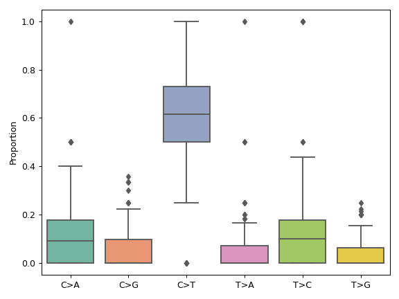
- plot_snvclss(samples=None, color=None, colormap=None, width=0.8, legend=True, flip=False, to_csv=None, ax=None, figsize=None, **kwargs)[source]
Create a bar plot showing the proportions of the six SNV classes for individual samples.
- Parameters:
samples (list, optional) – List of samples to display (in that order too). If samples that are absent in the MafFrame are provided, the method will give a warning but still draw an empty bar for those samples.
color (list, optional) – List of color tuples. See the Control plot colors tutorial for details.
colormap (str or matplotlib colormap object, optional) – Colormap to select colors from. See the Control plot colors tutorial for details.
width (float, default: 0.8) – The width of the bars.
legend (bool, default: True) – Place legend on axis subplots.
flip (bool, default: False) – If True, flip the x and y axes.
to_csv (str, optional) – Write the plot’s data to a CSV file.
ax (matplotlib.axes.Axes, optional) – Pre-existing axes for the plot. Otherwise, crete a new one.
figsize (tuple, optional) – Width, height in inches. Format: (float, float).
kwargs – Other keyword arguments will be passed down to
pandas.DataFrame.plot.bar()orpandas.DataFrame.plot.barh().
- Returns:
The matplotlib axes containing the plot.
- Return type:
matplotlib.axes.Axes
See also
MafFrame.plot_snvclscCreate a bar plot summarizing the count distrubtions of the six SNV classes for all samples.
MafFrame.plot_snvclspCreate a box plot summarizing the proportion distrubtions of the six SNV classes for all sample.
Examples
>>> import matplotlib.pyplot as plt
>>> from fuc import common, pymaf
>>> common.load_dataset('tcga-laml')
>>> maf_file = '~/fuc-data/tcga-laml/tcga_laml.maf.gz'
>>> mf = pymaf.MafFrame.from_file(maf_file)
>>> ax = mf.plot_snvclss(width=1, color=plt.get_cmap('Set2').colors)
>>> ax.legend(loc='upper right')
>>> plt.tight_layout()

- plot_summary(figsize=(15, 10), title_fontsize=16, ticklabels_fontsize=12, legend_fontsize=12)[source]
Create a summary figure for MafFrame.
- Parameters:
figsize (tuple, default: (15, 10)) – Width, height in inches. Format: (float, float).
title_fontsize (float, default: 16) – Font size of subplot titles.
ticklabels_fontsize (float, default: 12) – Font size of tick labels.
legend_fontsize (float, default: 12) – Font size of legend texts.
Examples
>>> import matplotlib.pyplot as plt
>>> from fuc import common, pymaf
>>> common.load_dataset('tcga-laml')
>>> maf_file = '~/fuc-data/tcga-laml/tcga_laml.maf.gz'
>>> mf = pymaf.MafFrame.from_file(maf_file)
>>> mf.plot_summary()
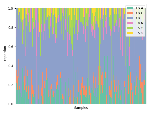
- plot_titv(af=None, group_col=None, group_order=None, flip=False, ax=None, figsize=None, **kwargs)[source]
Create a box plot showing the Ti/Tv proportions of samples.
- Parameters:
af (AnnFrame, optional) – AnnFrame containing sample annotation data.
group_col (str, optional) – AnnFrame column containing sample group information.
group_order (list, optional) – List of sample group names.
flip (bool, default: False) – If True, flip the x and y axes.
ax (matplotlib.axes.Axes, optional) – Pre-existing axes for the plot. Otherwise, crete a new one.
figsize (tuple, optional) – Width, height in inches. Format: (float, float).
kwargs – Other keyword arguments will be passed down to
seaborn.boxplot().
- Returns:
The matplotlib axes containing the plot.
- Return type:
matplotlib.axes.Axes
See also
fuc.api.pyvcf.VcfFrame.plot_titvSimilar method for the
fuc.api.pyvcf.VcfFrameclass.
Examples
Below is a simple example:
>>> import matplotlib.pyplot as plt
>>> from fuc import common, pymaf
>>> common.load_dataset('tcga-laml')
>>> maf_file = '~/fuc-data/tcga-laml/tcga_laml.maf.gz'
>>> mf = pymaf.MafFrame.from_file(maf_file)
>>> mf.plot_titv()
>>> plt.tight_layout()
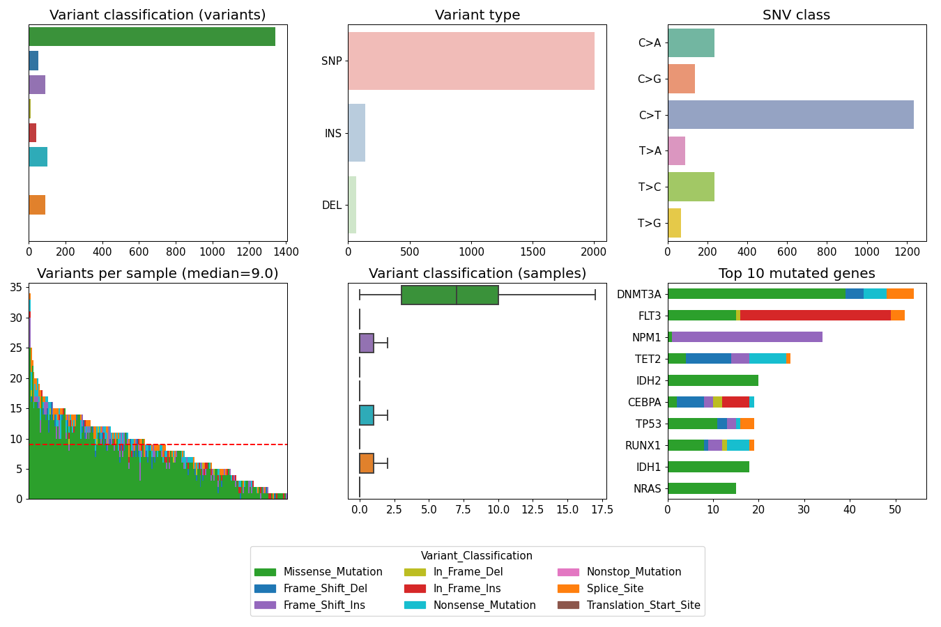
We can create a grouped bar plot based on FAB classification:
>>> annot_file = '~/fuc-data/tcga-laml/tcga_laml_annot.tsv'
>>> af = common.AnnFrame.from_file(annot_file, sample_col=0)
>>> mf.plot_titv(af=af,
...              group_col='FAB_classification',
...              group_order=['M0', 'M1', 'M2'])
>>> plt.tight_layout()

- plot_tmb(samples=None, width=0.8, ax=None, figsize=None, **kwargs)[source]
Create a bar plot showing the TMB distributions of samples.
- Parameters:
samples (list, optional) – List of samples to display (in that order too). If samples that are absent in the MafFrame are provided, the method will give a warning but still draw an empty bar for those samples.
width (float, default: 0.8) – The width of the bars.
ax (matplotlib.axes.Axes, optional) – Pre-existing axes for the plot. Otherwise, crete a new one.
figsize (tuple, optional) – Width, height in inches. Format: (float, float).
kwargs – Other keyword arguments will be passed down to
pandas.DataFrame.plot.bar().
- Returns:
The matplotlib axes containing the plot.
- Return type:
matplotlib.axes.Axes
Examples
Below is a simple example:
>>> import matplotlib.pyplot as plt
>>> from fuc import common, pymaf
>>> common.load_dataset('tcga-laml')
>>> maf_file = '~/fuc-data/tcga-laml/tcga_laml.maf.gz'
>>> mf = pymaf.MafFrame.from_file(maf_file)
>>> mf.plot_tmb(width=1)
>>> plt.tight_layout()

- plot_tmb_matched(af, patient_col, group_col, group_order=None, patients=None, legend=True, ax=None, figsize=None, **kwargs)[source]
Create a grouped bar plot showing TMB distributions for different group levels in each patient.
- Parameters:
af (AnnFrame) – AnnFrame containing sample annotation data.
patient_col (str) – AnnFrame column containing patient information.
group_col (str) – AnnFrame column containing sample group information.
group_order (list, optional) – List of sample group names.
patients (list, optional) – List of patient names.
legend (bool, default: True) – Place legend on axis subplots.
ax (matplotlib.axes.Axes, optional) – Pre-existing axes for the plot. Otherwise, crete a new one.
figsize (tuple, optional) – Width, height in inches. Format: (float, float).
kwargs – Other keyword arguments will be passed down to
pandas.DataFrame.plot.bar()
- Returns:
The matplotlib axes containing the plot.
- Return type:
matplotlib.axes.Axes
- plot_vaf(vaf_col, count=10, af=None, group_col=None, group_order=None, flip=False, sort=True, ax=None, figsize=None, **kwargs)[source]
Create a box plot showing the VAF distributions of top mutated genes.
A grouped box plot can be created with
group_col(requires an AnnFrame).- Parameters:
vaf_col (str) – MafFrame column containing VAF data.
count (int, default: 10) – Number of top mutated genes to display.
af (AnnFrame, optional) – AnnFrame containing sample annotation data.
group_col (str, optional) – AnnFrame column containing sample group information.
group_order (list, optional) – List of sample group names.
flip (bool, default: False) – If True, flip the x and y axes.
sort (bool, default: True) – If False, do not sort the genes by median value.
ax (matplotlib.axes.Axes, optional) – Pre-existing axes for the plot. Otherwise, crete a new one.
figsize (tuple, optional) – Width, height in inches. Format: (float, float).
kwargs – Other keyword arguments will be passed down to
seaborn.boxplot().
- Returns:
The matplotlib axes containing the plot.
- Return type:
matplotlib.axes.Axes
Examples
Below is a simple example:
>>> import matplotlib.pyplot as plt
>>> from fuc import common, pymaf
>>> common.load_dataset('tcga-laml')
>>> maf_file = '~/fuc-data/tcga-laml/tcga_laml.maf.gz'
>>> mf = pymaf.MafFrame.from_file(maf_file)
>>> mf.plot_vaf('i_TumorVAF_WU')
>>> plt.tight_layout()
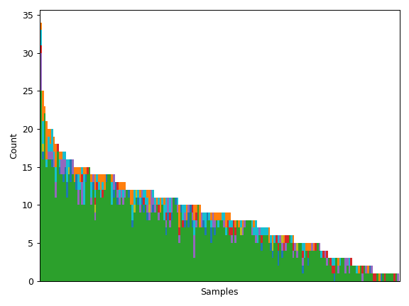
We can create a grouped bar plot based on FAB classification:
>>> annot_file = '~/fuc-data/tcga-laml/tcga_laml_annot.tsv'
>>> af = common.AnnFrame.from_file(annot_file, sample_col=0)
>>> mf.plot_vaf('i_TumorVAF_WU',
...             af=af,
...             group_col='FAB_classification',
...             group_order=['M1', 'M2', 'M3'],
...             count=5)
>>> plt.tight_layout()
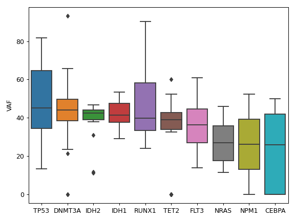
- plot_varcls(ax=None, figsize=None, **kwargs)[source]
Create a bar plot for the nonsynonymous variant classes.
- Parameters:
ax (matplotlib.axes.Axes, optional) – Pre-existing axes for the plot. Otherwise, crete a new one.
figsize (tuple, optional) – Width, height in inches. Format: (float, float).
kwargs – Other keyword arguments will be passed down to
matplotlib.axes.Axes.bar()andseaborn.barplot().
- Returns:
The matplotlib axes containing the plot.
- Return type:
matplotlib.axes.Axes
Examples
>>> import matplotlib.pyplot as plt
>>> from fuc import common, pymaf
>>> common.load_dataset('tcga-laml')
>>> maf_file = '~/fuc-data/tcga-laml/tcga_laml.maf.gz'
>>> mf = pymaf.MafFrame.from_file(maf_file)
>>> mf.plot_varcls()
>>> plt.tight_layout()
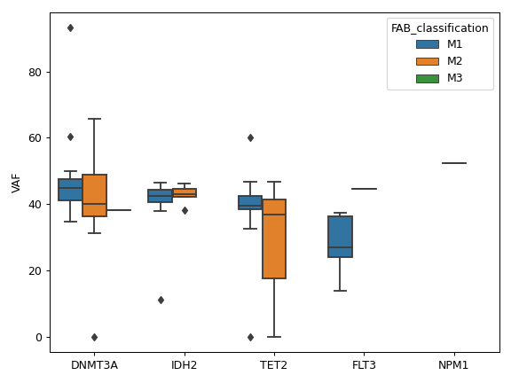
- plot_varsum(flip=False, ax=None, figsize=None)[source]
Create a summary box plot for variant classifications.
- Parameters:
flip (bool, default: False) – If True, flip the x and y axes.
ax (matplotlib.axes.Axes, optional) – Pre-existing axes for the plot. Otherwise, crete a new one.
figsize (tuple, optional) – Width, height in inches. Format: (float, float).
- Returns:
The matplotlib axes containing the plot.
- Return type:
matplotlib.axes.Axes
Examples
>>> import matplotlib.pyplot as plt
>>> from fuc import common, pymaf
>>> common.load_dataset('tcga-laml')
>>> maf_file = '~/fuc-data/tcga-laml/tcga_laml.maf.gz'
>>> mf = pymaf.MafFrame.from_file(maf_file)
>>> mf.plot_varsum()
>>> plt.tight_layout()
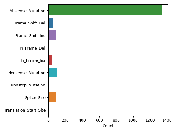
- plot_vartype(palette=None, flip=False, ax=None, figsize=None, **kwargs)[source]
Create a bar plot summarizing the count distrubtions of viaration types for all samples.
- Parameters:
palette (str, optional) – Name of the seaborn palette. See the Control plot colors tutorial for details.
flip (bool, default: False) – If True, flip the x and y axes.
ax (matplotlib.axes.Axes, optional) – Pre-existing axes for the plot. Otherwise, crete a new one.
figsize (tuple, optional) – Width, height in inches. Format: (float, float).
kwargs – Other keyword arguments will be passed down to
seaborn.barplot().
- Returns:
The matplotlib axes containing the plot.
- Return type:
matplotlib.axes.Axes
Examples
>>> import matplotlib.pyplot as plt
>>> from fuc import common, pymaf
>>> common.load_dataset('tcga-laml')
>>> maf_file = '~/fuc-data/tcga-laml/tcga_laml.maf.gz'
>>> mf = pymaf.MafFrame.from_file(maf_file)
>>> mf.plot_vartype()
>>> plt.tight_layout()
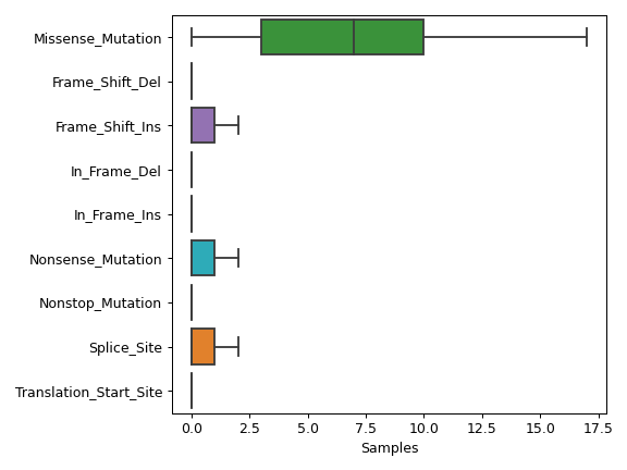
- plot_waterfall(count=10, keep_empty=False, samples=None, ax=None, figsize=None, **kwargs)[source]
Create a waterfall plot (oncoplot).
See this tutorial to learn how to create customized oncoplots.
- Parameters:
count (int, default: 10) – Number of top mutated genes to display.
keep_empty (bool, default: False) – If True, display samples that do not have any mutations.
samples (list, optional) – List of samples to display (in that order too). If samples that are absent in the MafFrame are provided, the method will give a warning but still draw an empty bar for those samples.
ax (matplotlib.axes.Axes, optional) – Pre-existing axes for the plot. Otherwise, crete a new one.
figsize (tuple, optional) – Width, height in inches. Format: (float, float).
kwargs – Other keyword arguments will be passed down to
seaborn.heatmap().
- Returns:
The matplotlib axes containing the plot.
- Return type:
matplotlib.axes.Axes
Examples
>>> import matplotlib.pyplot as plt
>>> from fuc import common, pymaf
>>> common.load_dataset('tcga-laml')
>>> maf_file = '~/fuc-data/tcga-laml/tcga_laml.maf.gz'
>>> mf = pymaf.MafFrame.from_file(maf_file)
>>> mf.plot_waterfall(linewidths=0.5)
>>> plt.tight_layout()
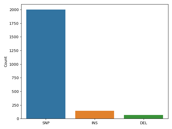
- plot_waterfall_matched(af, patient_col, group_col, group_order, count=10, ax=None, figsize=None)[source]
Create a waterfall plot using matched samples from each patient.
- Parameters:
af (AnnFrame) – AnnFrame containing sample annotation data.
patient_col (str) – AnnFrame column containing patient information.
group_col (str) – AnnFrame column containing sample group information.
group_order (list) – List of sample group names.
count (int, default: 10) – Number of top mutated genes to include.
ax (matplotlib.axes.Axes, optional) – Pre-existing axes for the plot. Otherwise, crete a new one.
figsize (tuple, optional) – Width, height in inches. Format: (float, float).
- Returns:
The matplotlib axes containing the plot.
- Return type:
matplotlib.axes.Axes
- property samples
List of the sample names.
- Type:
list
- property shape
Dimensionality of MafFrame (variants, samples).
- Type:
tuple
- subset(samples, exclude=False)[source]
Subset MafFrame for specified samples.
- Parameters:
samples (str, list, or pandas.Series) – Sample name or list of names (the order does not matters).
exclude (bool, default: False) – If True, exclude specified samples.
- Returns:
Subsetted MafFrame.
- Return type:
Examples
>>> from fuc import common, pymaf
>>> common.load_dataset('tcga-laml')
>>> maf_file = '~/fuc-data/tcga-laml/tcga_laml.maf.gz'
>>> mf = pymaf.MafFrame.from_file(maf_file)
>>> mf.shape
(2207, 193)
>>> mf.subset(['TCGA-AB-2988', 'TCGA-AB-2869']).shape
(27, 2)
>>> mf.subset(['TCGA-AB-2988', 'TCGA-AB-2869'], exclude=True).shape
(2180, 191)
- to_string()[source]
Render MafFrame to a console-friendly tabular output.
- Returns:
String representation of MafFrame.
- Return type:
str
- to_vcf(fasta=None, ignore_indels=False, cols=None, names=None)[source]
Write the MafFrame to a sorted VcfFrame.
Converting from MAF to VCF is pretty straightforward for SNVs, but it can be challenging for INDELs and complex events involving multiple nucleotides (e.g. ‘AAGG’ → ‘CCCG’). This is because, for the latter case we need to identify the “anchor” nucleotide for each event, which is crucial for constructing a properly formatted VCF. For example, a deletion event ‘AGT’ → ‘-’ in MAF would have to be converted to ‘CAGT’ → ‘C’ in the VCF where ‘C’ is our anchor nucleotide. The position should be shifted by one as well.
In order to tackle this issue, the method makes use of a reference assembly (i.e. FASTA file). If SNVs are your only concern, then you do not need a FASTA file and can just set
ignore_indelsas True. If you are going to provide a FASTA file, please make sure to select the appropriate one (e.g. one that matches the genome assembly). For example, if your MAF is in hg19/GRCh37, use the ‘hs37d5.fa’ file which can be freely downloaded from the 1000 Genomes Project.- Parameters:
fasta (str, optional) – FASTA file. Required if
ignore_indelsis False.ignore_indels (bool, default: False) – If True, do not include INDELs in the VcfFrame. Useful when a FASTA file is not available.
cols (str or list, optional) – Column(s) in the MafFrame which contain additional genotype data of interest. If provided, these data will be added to individual sample genotypes (e.g. ‘0/1:0.23’).
names (str or list, optional) – Name(s) to be displayed in the FORMAT field (e.g. AD, AF, DP). If not provided, the original column name(s) will be displayed.
- Returns:
VcfFrame object.
- Return type:
Examples
>>> from fuc import pymaf
>>> mf = pymaf.MafFrame.from_file('in.maf')
>>> vf = mf.to_vcf(fasta='hs37d5.fa')
>>> vf = mf.to_vcf(ignore_indels=True)
>>> vf = mf.to_vcf(fasta='hs37d5.fa', cols='i_TumorVAF_WU', names='AF')
- variants()[source]
List unique variants in MafFrame.
- Returns:
List of unique variants.
- Return type:
list
Examples
>>> from fuc import common, pymaf
>>> common.load_dataset('tcga-laml')
>>> maf_file = '~/fuc-data/tcga-laml/tcga_laml.maf.gz'
>>> mf = pymaf.MafFrame.from_file(maf_file)
>>> mf.variants()[:5]
['1:1571791:1571791:G:A', '1:1747228:1747228:T:G', '1:2418350:2418350:C:T', '1:3328523:3328523:G:A', '1:3638739:3638739:C:T']
fuc.pysnpeff
The pysnpeff submodule is designed for parsing VCF annotation data from
the SnpEff program. It should be
used with pyvcf.VcfFrame.
One VCF record can have several SnpEff annotations if, for example, the record is a multiallelic site or the variant is shared by multiple genes. When more than one annotations are reported, SnpEff will sort them by their importance. For more details, visit the official website.
For each annotation, SnpEff provides the following data:
Allele - ALT allele.
Annotation - Sequence Ontology terms concatenated using ‘&’.
Annotation_Impact - HIGH, MODERATE, LOW, or MODIFIER.
Gene_Name - Common gene name (HGNC).
Gene_ID - Gene ID.
Feature_Type - Which type of feature is in the next field.
Feature_ID - Transcript ID, Motif ID, miRNA, ChipSeq peak, etc.
Transcript_BioType - Coding or noncoding.
Rank - Exon or Intron rank / total number of exons or introns.
HGVS.c - Variant using HGVS notation (DNA level).
HGVS.p - Variant using HGVS notation (Protein level).
cDNA.pos / cDNA.length - Position in cDNA and trancript’s cDNA length.
CDS.pos / CDS.length - Position and number of coding bases.
AA.pos / AA.length - Position and number of AA.
Distance - All items in this field are options.
ERRORS / WARNINGS - Messages that can affect annotation accuracy.
INFO - Additional information.
Functions:
|
Filter out rows based on the SnpEff annotations. |
|
Parse SnpEff annotations. |
|
Return the first SnpEff annotation for the row. |
- fuc.api.pysnpeff.filter_ann(vf, targets, include=True)[source]
Filter out rows based on the SnpEff annotations.
- Parameters:
vf (fuc.api.pyvcf.VcfFrame) – Input VcfFrame.
targets (list) – List of annotations (e.g. [‘missense_variant’, ‘stop_gained’]).
include (bool, default: False) – If True, include only such rows instead of excluding them.
- Returns:
vf – Filtered VcfFrame.
- Return type:
- fuc.api.pysnpeff.parseann(vf, idx, sep=' | ')[source]
Parse SnpEff annotations.
- Parameters:
vf (fuc.api.pyvcf.VcfFrame) – Input VcfFrame.
i (list) – List of annotation indicies.
sep (str, default: ‘ | ‘) – Separator for joining requested annotations.
- Returns:
s – Parsed annotations.
- Return type:
pandas.Series
fuc.pyvcf
The pyvcf submodule is designed for working with VCF files. It implements
pyvcf.VcfFrame which stores VCF data as pandas.DataFrame to allow
fast computation and easy manipulation. The pyvcf.VcfFrame class also
contains many useful plotting methods such as VcfFrame.plot_comparison
and VcfFrame.plot_tmb. The submodule strictly adheres to the
standard VCF specification.
A typical VCF file contains metadata lines (prefixed with ‘##’), a header line (prefixed with ‘#’), and genotype lines that begin with a chromosome identifier (e.g. ‘chr1’). See the VCF specification above for an example VCF file.
Genotype lines usually consist of nine columns for storing variant information (all fixed and mandatory except for the FORMAT column) plus additional sample-specific columns for expressing individual genotype calls (e.g. ‘0/1’). Missing values are allowed in some cases and can be specified with a dot (‘.’). The first nine columns are:
No. |
Column |
Description |
Required |
Missing |
Examples |
|---|---|---|---|---|---|
1 |
CHROM |
Chromosome or contig identifier |
✅ |
❌ |
‘chr2’, ‘2’, ‘chrM’ |
2 |
POS |
1-based reference position |
✅ |
❌ |
10041, 23042 |
3 |
ID |
‘;’-separated variant identifiers |
✅ |
✅ |
‘.’, ‘rs35’, ‘rs9;rs53’ |
4 |
REF |
Reference allele |
✅ |
❌ |
‘A’, ‘GT’ |
5 |
ALT |
‘,’-separated alternate alleles |
✅ |
❌ |
‘T’, ‘ACT’, ‘C,T’ |
6 |
QUAL |
Phred-scaled quality score for ALT |
✅ |
✅ |
‘.’, 67, 12 |
7 |
FILTER |
‘;’-separated filters that failed |
✅ |
✅ |
‘.’, ‘PASS’, ‘q10;s50’ |
8 |
INFO |
‘;’-separated information fields |
✅ |
✅ |
‘.’, ‘DP=14;AF=0.5;DB’ |
9 |
FORMAT |
‘:’-separated genotype fields |
❌ |
❌ |
‘GT’, ‘GT:AD:DP’ |
You will sometimes come across VCF files that have only eight columns, and do not contain the FORMAT column or sample-specific information. These are called “sites-only” VCF files, and normally represent genetic variation that has been observed in a large population. Generally, information about the population of origin should be included in the header. Note that the pyvcf submodule supports these sites-only VCF files as well.
There are several reserved keywords in the INFO and FORMAT columns that are standards across the community. Popular keywords are listed below:
Column |
Key |
Number |
Type |
Description |
|---|---|---|---|---|
INFO |
AC |
A |
Integer |
Allele count in genotypes, for each ALT allele, in the same order as listed |
INFO |
AN |
1 |
Integer |
Total number of alleles in called genotypes |
INFO |
AF |
A |
Float |
Allele frequency for each ALT allele in the same order as listed (estimated from primary data, not called genotypes) |
FORMAT |
AD |
R |
Integer |
Total read depth for each allele |
FORMAT |
AF |
1 |
Float |
Allele fraction of the event in the tumor |
FORMAT |
DP |
1 |
Integer |
Read depth |
If sample annotation data are available for a given VCF file, use
the common.AnnFrame class to import the data.
Classes:
|
Class for storing VCF data. |
Functions:
|
Call SNVs and indels from BAM files. |
For given genotype, return its diploid form. |
|
|
For given genotype, return True if it has variation. |
|
For given genotype, return True if it is heterozygous. |
|
For given genotype, return True if it has missing value. |
|
For given genotype, return its ploidy number. |
|
For given genotype, return True if it is polyploid. |
For given genotype, return its pseudophased form. |
|
|
For given genotype, return its unphased form. |
|
Return True if all of the sampled contigs from a VCF file have the (annoying) 'chr' string. |
|
Merge VcfFrame objects. |
|
Create a scatter plot showing the correlation of allele frequency between two VCF files. |
|
Rescue filtered variants if they are PASS in at least one of the input VCF files. |
|
For given row, return AC/AN/AF calculation for INFO column. |
|
For given row, return True if it has indel. |
|
For given row, return formatted missing genotype. |
|
For given row, return requested data from INFO column. |
|
For given row, return True if all genotypes are phased. |
|
For given row, return updated data from INFO column. |
|
Slice a VCF file for specified regions. |
|
Split VcfFrame by individual. |
- class fuc.api.pyvcf.VcfFrame(meta, df)[source]
Class for storing VCF data.
Sites-only VCF files are supported.
- Parameters:
meta (list) – List of metadata lines.
df (pandas.DataFrame) – DataFrame containing VCF data.
See also
VcfFrame.from_dictConstruct VcfFrame from a dict of array-like or dicts.
VcfFrame.from_fileConstruct VcfFrame from a VCF file.
VcfFrame.from_stringConstruct VcfFrame from a string.
Examples
Constructing VcfFrame from pandas DataFrame:
>>> from fuc import pyvcf
>>> import pandas as pd
>>> data = {
...     'CHROM': ['chr1', 'chr1', 'chr1'],
...     'POS': [100, 101, 102],
...     'ID': ['.', '.', '.',],
...     'REF': ['G', 'T', 'A'],
...     'ALT': ['A', 'C', 'T'],
...     'QUAL': ['.', '.', '.'],
...     'FILTER': ['.', '.', '.'],
...     'INFO': ['.', '.', '.'],
...     'FORMAT': ['GT', 'GT', 'GT'],
...     'Steven': ['0/1', '0/1', '0/1'],
... }
>>> df = pd.DataFrame(data)
>>> vf = pyvcf.VcfFrame(['##fileformat=VCFv4.3'], df)
>>> vf.meta
['##fileformat=VCFv4.3']
>>> vf.df
  CHROM  POS ID REF ALT QUAL FILTER INFO FORMAT Steven
0  chr1  100  .   G   A    .      .    .     GT    0/1
1  chr1  101  .   T   C    .      .    .     GT    0/1
2  chr1  102  .   A   T    .      .    .     GT    0/1
Methods:
add_af([decimals])Compute AF from AD and then add it to the FORMAT field.
add_dp()Compute DP using AD and add it to the FORMAT field.
add_flag(flag[, order, index])Add the given flag to the INFO field.
calculate_concordance(a, b[, c, mode])Calculate genotype concordance between two (A, B) or three (A, B, C) samples.
collapse()Collapse duplicate records in the VcfFrame.
combine(a, b)Combine genotype data from two samples (A, B).
compare(other)Compare to another VcfFrame and show the differences in genotype calling.
compute_info(key)Compute AC/AN/AF for INFO column.
copy()Return a copy of the VcfFrame.
copy_df()Return a copy of the dataframe.
Return a copy of the metadata.
Diploidize VcfFrame.
drop_duplicates([subset, keep])Return VcfFrame with duplicate rows removed.
duplicated([subset, keep])Return boolean Series denoting duplicate rows in VcfFrame.
empty_samples([threshold, opposite, as_list])Remove samples with high missingness.
expand()Expand each multiallelic locus to multiple rows.
extract_format(k[, func, as_nan])Extract data for the specified FORMAT key.
extract_info(k[, func, as_nan])Extract data for the specified INFO key.
fetch(variant)Fetch the VCF row that matches specified variant.
filter_bed(bed[, opposite, as_index])Filter rows intersecting with given BED.
filter_empty([threshold, opposite, as_index])Filter rows with high missingness.
filter_flagall(flags[, opposite, as_index])Filter rows with all given INFO flags.
filter_flagany(flags[, opposite, as_index])Filter rows with any given INFO flags.
filter_gsa([opposite, as_index])Filter rows specific to Illumina's GSA array.
filter_indel([opposite, as_index])Filter rows with indel.
filter_multialt([opposite, as_index])Filter rows with multiple ALT alleles.
filter_pass([opposite, as_index])Filter rows with PASS in FILTER column.
filter_phased([opposite, as_index])Filter rows with phased genotypes.
filter_polyp([opposite, as_index])Filter rows with polyploid genotypes.
filter_qual(threshold[, opposite, as_index])Filter rows with low QUAL values.
filter_sampall([samples, opposite, as_index])Filter rows where all given samples have variant.
filter_sampany([samples, opposite, as_index])Filter rows where any given samples have variant.
filter_sampnum(threshold[, opposite, as_index])Filter rows with high variant prevalence.
filter_vcf(vcf[, opposite, as_index])Filter rows intersecting with given VCF.
from_dict(meta, data)Construct VcfFrame from a dict of array-like or dicts.
from_file(fn[, compression, meta_only, regions])Construct VcfFrame from a VCF file.
from_string(s[, meta_only])Construct VcfFrame from a string.
get_af(sample, variant)Get allele fraction for a pair of sample and variant.
markmiss(expr[, greedy, opposite, samples, ...])Mark all genotypes that satisfy the query expression as missing.
merge(other[, how, format, sort, collapse])Merge with the other VcfFrame.
Print metadata lines with a key.
miss2ref()Convert missing genotype (./.) to homozygous REF (0/0).
plot_comparison(a, b[, c, labels, ax, figsize])Create a Venn diagram showing genotype concordance between groups.
plot_hist_format(k[, af, group_col, ...])Create a histogram showing the distribution of data for the specified FORMAT key.
plot_hist_info(k[, kde, ax, figsize])Create a histogram showing the distribution of data for the specified INFO key.
plot_rainfall(sample[, palette, ax, ...])Create a rainfall plot visualizing inter-variant distance on a linear genomic scale for single sample.
plot_region(sample[, k, color, region, ...])Create a scatter plot showing read depth profile of a sample for the specified region.
plot_regplot_tmb(a, b[, ax, figsize])Create a scatter plot with a linear regression model fit visualizing correlation between TMB in two sample groups.
plot_snvclsc([af, group_col, group_order, ...])Create a bar plot summarizing the count distrubtions of the six SNV classes for all samples.
plot_snvclsp([af, group_col, group_order, ...])Create a box plot summarizing the proportion distrubtions of the six SNV classes for all sample.
plot_snvclss([color, colormap, width, ...])Create a bar plot showing the proportions of the six SNV classes for individual samples.
plot_titv([af, group_col, group_order, ...])Create a box plot showing the Ti/Tv proportions of samples.
plot_tmb([af, group_col, group_order, kde, ...])Create a histogram showing TMB distribution.
Pseudophase VcfFrame.
rename(names[, indicies])Rename the samples.
slice(region)Slice VcfFrame for specified region.
sort()Sort the VcfFrame by chromosome and position.
strip([format, metadata])Remove any unnecessary data.
subset(samples[, exclude])Subset VcfFrame for specified samples.
subtract(a, b)Subtract genotype data between two samples (A, B).
to_bed()Convert VcfFrame to BedFrame.
to_file(fn[, compression])Write VcfFrame to a VCF file.
Render the VcfFrame to a console-friendly tabular output.
List unique variants in VcfFrame.
unphase()Unphase all the sample genotypes.
update_chr_prefix([mode])Add or remove the (annoying) 'chr' string from the CHROM column.
Attributes:
List of contig names.
DataFrame containing VCF data.
Indicator whether VcfFrame is empty.
Whether the (annoying) 'chr' string is found.
List of metadata lines.
Return True if every genotype in VcfFrame is haplotype phased.
List of sample names.
Dimensionality of VcfFrame (variants, samples).
Whether the VCF is sites-only.
- add_af(decimals=3)[source]
Compute AF from AD and then add it to the FORMAT field.
This method will compute allele fraction for each ALT allele in the same order as listed.
- Parameters:
decimals (int, default: 3) – Number of decimals to display.
- Returns:
Updated VcfFrame object.
- Return type:
Examples
>>> from fuc import pyvcf
>>> data = {
...     'CHROM': ['chr1', 'chr1', 'chr1', 'chr1'],
...     'POS': [100, 101, 102, 103],
...     'ID': ['.', '.', '.', '.'],
...     'REF': ['A', 'G', 'A', 'C'],
...     'ALT': ['C', 'T', 'G', 'G,A'],
...     'QUAL': ['.', '.', '.', '.'],
...     'FILTER': ['.', '.', '.', '.'],
...     'INFO': ['.', '.', '.', '.'],
...     'FORMAT': ['GT:AD', 'GT:AD', 'GT', 'GT:AD'],
...     'A': ['0/1:12,15', '0/0:32,1', '0/1', './.:.'],
...     'B': ['0/1:13,17', '0/1:14,15', './.', '1/2:0,11,17'],
... }
>>> vf = pyvcf.VcfFrame.from_dict([], data)
>>> vf.df
  CHROM  POS ID REF  ALT QUAL FILTER INFO FORMAT          A            B
0  chr1  100  .   A    C    .      .    .  GT:AD  0/1:12,15    0/1:13,17
1  chr1  101  .   G    T    .      .    .  GT:AD   0/0:32,1    0/1:14,15
2  chr1  102  .   A    G    .      .    .     GT        0/1          ./.
3  chr1  103  .   C  G,A    .      .    .  GT:AD      ./.:.  1/2:0,11,17
>>> vf.add_af().df
  CHROM  POS ID REF  ALT QUAL FILTER INFO    FORMAT                      A                              B
0  chr1  100  .   A    C    .      .    .  GT:AD:AF  0/1:12,15:0.444,0.556          0/1:13,17:0.433,0.567
1  chr1  101  .   G    T    .      .    .  GT:AD:AF   0/0:32,1:0.970,0.030          0/1:14,15:0.483,0.517
2  chr1  102  .   A    G    .      .    .     GT:AF                  0/1:.                          ./.:.
3  chr1  103  .   C  G,A    .      .    .  GT:AD:AF                ./.:.:.  1/2:0,11,17:0.000,0.393,0.607
- add_dp()[source]
Compute DP using AD and add it to the FORMAT field.
- Returns:
Updated VcfFrame.
- Return type:
Examples
Assume we have the following data:
>>> from fuc import pyvcf
>>> data = {
...     'CHROM': ['chr1', 'chr1', 'chr2', 'chr2'],
...     'POS': [100, 100, 200, 200],
...     'ID': ['.', '.', '.', '.'],
...     'REF': ['A', 'A', 'C', 'C'],
...     'ALT': ['C', 'T', 'G', 'G,A'],
...     'QUAL': ['.', '.', '.', '.'],
...     'FILTER': ['.', '.', '.', '.'],
...     'INFO': ['.', '.', '.', '.'],
...     'FORMAT': ['GT:AD', 'GT:AD', 'GT:AD', 'GT:AD'],
...     'Steven': ['0/1:12,15', '0/0:32,1', '0/1:16,12', './.:.'],
...     'Sara': ['0/1:13,17', '0/1:14,15', './.:.', '1/2:0,11,17'],
... }
>>> vf = pyvcf.VcfFrame.from_dict([], data)
>>> vf.df
  CHROM  POS ID REF  ALT QUAL FILTER INFO FORMAT     Steven         Sara
0  chr1  100  .   A    C    .      .    .  GT:AD  0/1:12,15    0/1:13,17
1  chr1  100  .   A    T    .      .    .  GT:AD   0/0:32,1    0/1:14,15
2  chr2  200  .   C    G    .      .    .  GT:AD  0/1:16,12        ./.:.
3  chr2  200  .   C  G,A    .      .    .  GT:AD      ./.:.  1/2:0,11,17
We can add the DP subfield to our genotype data:
>>> vf.add_dp().df
  CHROM  POS ID REF  ALT QUAL FILTER INFO    FORMAT        Steven            Sara
0  chr1  100  .   A    C    .      .    .  GT:AD:DP  0/1:12,15:27    0/1:13,17:30
1  chr1  100  .   A    T    .      .    .  GT:AD:DP   0/0:32,1:33    0/1:14,15:29
2  chr2  200  .   C    G    .      .    .  GT:AD:DP  0/1:16,12:28         ./.:.:.
3  chr2  200  .   C  G,A    .      .    .  GT:AD:DP       ./.:.:.  1/2:0,11,17:28
- add_flag(flag, order='last', index=None)[source]
Add the given flag to the INFO field.
The default behavior is to add the flag to all rows in the VcfFrame.
- Parameters:
flag (str) – INFO flag.
order ({‘last’, ‘first’, False}, default: ‘last’) – Determines the order in which the flag will be added.
last: Add to the end of the list.first: Add to the beginning of the list.False: Overwrite the existing field.
index (list or pandas.Series, optional) – Boolean index array indicating which rows should be updated.
- Returns:
Updated VcfFrame.
- Return type:
Examples
Assume we have the following data:
>>> from fuc import pyvcf
>>> data = {
...     'CHROM': ['chr1', 'chr1', 'chr1', 'chr1'],
...     'POS': [100, 101, 102, 103],
...     'ID': ['.', '.', '.', '.'],
...     'REF': ['G', 'T', 'A', 'C'],
...     'ALT': ['A', 'C', 'T', 'A'],
...     'QUAL': ['.', '.', '.', '.'],
...     'FILTER': ['.', '.', '.', '.'],
...     'INFO': ['.', 'DB', 'DB', '.'],
...     'FORMAT': ['GT', 'GT', 'GT', 'GT'],
...     'Steven': ['0/0', '0/1', '0/1', '1/1'],
... }
>>> vf = pyvcf.VcfFrame.from_dict([], data)
>>> vf.df
  CHROM  POS ID REF ALT QUAL FILTER INFO FORMAT Steven
0  chr1  100  .   G   A    .      .    .     GT    0/0
1  chr1  101  .   T   C    .      .   DB     GT    0/1
2  chr1  102  .   A   T    .      .   DB     GT    0/1
3  chr1  103  .   C   A    .      .    .     GT    1/1
We can add the SOMATIC flag to the INFO field:
>>> vf.add_flag('SOMATIC').df
  CHROM  POS ID REF ALT QUAL FILTER        INFO FORMAT Steven
0  chr1  100  .   G   A    .      .     SOMATIC     GT    0/0
1  chr1  101  .   T   C    .      .  DB;SOMATIC     GT    0/1
2  chr1  102  .   A   T    .      .  DB;SOMATIC     GT    0/1
3  chr1  103  .   C   A    .      .     SOMATIC     GT    1/1
Setting
order='first'will append the flag at the beginning:>>> vf.add_flag('SOMATIC', order='first').df CHROM POS ID REF ALT QUAL FILTER INFO FORMAT Steven 0 chr1 100 . G A . . SOMATIC GT 0/0 1 chr1 101 . T C . . SOMATIC;DB GT 0/1 2 chr1 102 . A T . . SOMATIC;DB GT 0/1 3 chr1 103 . C A . . SOMATIC GT 1/1
Setting
order=Falsewill overwrite the INFO field:>>> vf.add_flag('SOMATIC', order=False).df CHROM POS ID REF ALT QUAL FILTER INFO FORMAT Steven 0 chr1 100 . G A . . SOMATIC GT 0/0 1 chr1 101 . T C . . SOMATIC GT 0/1 2 chr1 102 . A T . . SOMATIC GT 0/1 3 chr1 103 . C A . . SOMATIC GT 1/1
We can also specify which rows should be updated:
>>> vf.add_flag('SOMATIC', index=[True, True, False, False]).df
  CHROM  POS ID REF ALT QUAL FILTER        INFO FORMAT Steven
0  chr1  100  .   G   A    .      .     SOMATIC     GT    0/0
1  chr1  101  .   T   C    .      .  DB;SOMATIC     GT    0/1
2  chr1  102  .   A   T    .      .          DB     GT    0/1
3  chr1  103  .   C   A    .      .           .     GT    1/1
- calculate_concordance(a, b, c=None, mode='all')[source]
Calculate genotype concordance between two (A, B) or three (A, B, C) samples.
This method will return (Ab, aB, AB, ab) for comparison between two samples and (Abc, aBc, ABc, abC, AbC, aBC, ABC, abc) for three samples. Note that the former is equivalent to (FP, FN, TP, TN) if we assume A is the test sample and B is the truth sample.
Only biallelic sites will be used for calculation. Additionally, the method will ignore zygosity and only consider presence or absence of variant calls (e.g.
0/1and1/1will be treated the same).- Parameters:
a, b (str or int) – Name or index of Samples A and B.
c (str or int, optional) – Name or index of Sample C.
mode ({‘all’, ‘snv’, ‘indel’}, default: ‘all’) – Determines which variant types should be analyzed:
‘all’: Include both SNVs and INDELs.
‘snv’: Include SNVs only.
‘indel’: Include INDELs only.
- Returns:
Four- or eight-element tuple depending on the number of samples.
- Return type:
tuple
See also
fuc.api.common.sumstatReturn various summary statistics from (FP, FN, TP, TN).
Examples
Assume we have the following data:
>>> from fuc import pyvcf
>>> data = {
...     'CHROM': ['chr1', 'chr1', 'chr1', 'chr1', 'chr1'],
...     'POS': [100, 101, 102, 103, 104],
...     'ID': ['.', '.', '.', '.', '.'],
...     'REF': ['G', 'CT', 'T', 'C', 'A'],
...     'ALT': ['A', 'C', 'A', 'T', 'G,C'],
...     'QUAL': ['.', '.', '.', '.', '.'],
...     'FILTER': ['.', '.', '.', '.', '.'],
...     'INFO': ['.', '.', '.', '.', '.'],
...     'FORMAT': ['GT', 'GT', 'GT', 'GT', 'GT'],
...     'A': ['0/1', '0/0', '0/0', '0/1', '0/0'],
...     'B': ['1/1', '0/1', './.', '0/1', '0/0'],
...     'C': ['0/1', '0/1', '1/1', './.', '1/2'],
... }
>>> vf = pyvcf.VcfFrame.from_dict([], data)
>>> vf.df
  CHROM  POS ID REF  ALT QUAL FILTER INFO FORMAT    A    B    C
0  chr1  100  .   G    A    .      .    .     GT  0/1  1/1  0/1
1  chr1  101  .  CT    C    .      .    .     GT  0/0  0/1  0/1
2  chr1  102  .   T    A    .      .    .     GT  0/0  ./.  1/1
3  chr1  103  .   C    T    .      .    .     GT  0/1  0/1  ./.
4  chr1  104  .   A  G,C    .      .    .     GT  0/0  0/0  1/2
We can first compare the samples A and B:
>>> vf.calculate_concordance('A', 'B', mode='all')
(0, 1, 2, 1)
>>> vf.calculate_concordance('A', 'B', mode='snv')
(0, 0, 2, 1)
>>> vf.calculate_concordance('A', 'B', mode='indel')
(0, 1, 0, 0)
We can also compare all three samples at once:
>>> vf.calculate_concordance('A', 'B', 'C')
(0, 0, 1, 1, 0, 1, 1, 0)
- collapse()[source]
Collapse duplicate records in the VcfFrame.
Duplicate records have the identical values for CHROM, POS, and REF. They can result from merging two VCF files.
Note
The method will sort the order of ALT alleles.
- Returns:
Collapsed VcfFrame.
- Return type:
Examples
Assume we have the following data:
>>> from fuc import pyvcf
>>> data = {
...     'CHROM': ['chr1', 'chr1', 'chr2', 'chr2'],
...     'POS': [100, 100, 200, 200],
...     'ID': ['.', '.', '.', '.'],
...     'REF': ['A', 'A', 'C', 'C'],
...     'ALT': ['C', 'T', 'G', 'G,A'],
...     'QUAL': ['.', '.', '.', '.'],
...     'FILTER': ['.', '.', '.', '.'],
...     'INFO': ['.', '.', '.', '.'],
...     'FORMAT': ['GT:AD', 'GT:AD', 'GT:AD', 'GT:AD'],
...     'Steven': ['0/1:12,15', './.:.', '0/1:16,12', './.:.'],
...     'Sara': ['./.:.', '0/1:14,15', './.:.', '1/2:0,11,17'],
... }
>>> vf = pyvcf.VcfFrame.from_dict([], data)
>>> vf.df
  CHROM  POS ID REF  ALT QUAL FILTER INFO FORMAT     Steven         Sara
0  chr1  100  .   A    C    .      .    .  GT:AD  0/1:12,15        ./.:.
1  chr1  100  .   A    T    .      .    .  GT:AD      ./.:.    0/1:14,15
2  chr2  200  .   C    G    .      .    .  GT:AD  0/1:16,12        ./.:.
3  chr2  200  .   C  G,A    .      .    .  GT:AD      ./.:.  1/2:0,11,17
We collapse the VcfFrame:
>>> vf.collapse().df
  CHROM  POS ID REF  ALT QUAL FILTER INFO FORMAT       Steven         Sara
0  chr1  100  .   A  C,T    .      .    .  GT:AD  0/1:12,15,0  0/2:14,0,15
2  chr2  200  .   C  A,G    .      .    .  GT:AD  0/2:16,0,12  1/2:0,17,11
- combine(a, b)[source]
Combine genotype data from two samples (A, B).
This method can be especially useful when you want to consolidate genotype data from replicate samples. See examples below for more details.
- Parameters:
a, b (str or int) – Name or index of Samples A and B.
- Returns:
Resulting VCF column.
- Return type:
pandas.Series
See also
VcfFrame.subtractSubtract genotype data between two samples (A, B).
Examples
Assume we have following data where a cancer patient’s tissue sample has been sequenced twice:
>>> from fuc import pyvcf
>>> data = {
...     'CHROM': ['chr1', 'chr1', 'chr1', 'chr1', 'chr1'],
...     'POS': [100, 101, 102, 103, 104],
...     'ID': ['.', '.', '.', '.', '.'],
...     'REF': ['G', 'T', 'T', 'A', 'C'],
...     'ALT': ['A', 'C', 'A', 'C', 'G'],
...     'QUAL': ['.', '.', '.', '.', '.'],
...     'FILTER': ['.', '.', '.', '.', '.'],
...     'INFO': ['.', '.', '.', '.', '.'],
...     'FORMAT': ['GT:DP', 'GT:DP', 'GT:DP', 'GT:DP', 'GT:DP'],
...     'Tissue1': ['./.:.', '0/0:7', '0/1:28', '0/1:4', '0/1:32'],
...     'Tissue2': ['0/1:24', '0/1:42', './.:.', './.:.', '0/1:19'],
... }
>>> vf = pyvcf.VcfFrame.from_dict([], data)
>>> vf.df
  CHROM  POS ID REF ALT QUAL FILTER INFO FORMAT Tissue1 Tissue2
0  chr1  100  .   G   A    .      .    .  GT:DP   ./.:.  0/1:24
1  chr1  101  .   T   C    .      .    .  GT:DP   0/0:7  0/1:42
2  chr1  102  .   T   A    .      .    .  GT:DP  0/1:28   ./.:.
3  chr1  103  .   A   C    .      .    .  GT:DP   0/1:4   ./.:.
4  chr1  104  .   C   G    .      .    .  GT:DP  0/1:32  0/1:19
We can combine genotype data from ‘Tissue1’ and ‘Tissue2’ to get a more comprehensive variant profile:
>>> vf.df['Combined'] = vf.combine('Tissue1', 'Tissue2')
>>> vf.df
  CHROM  POS ID REF ALT QUAL FILTER INFO FORMAT Tissue1 Tissue2 Combined
0  chr1  100  .   G   A    .      .    .  GT:DP   ./.:.  0/1:24   0/1:24
1  chr1  101  .   T   C    .      .    .  GT:DP   0/0:7  0/1:42   0/1:42
2  chr1  102  .   T   A    .      .    .  GT:DP  0/1:28   ./.:.   0/1:28
3  chr1  103  .   A   C    .      .    .  GT:DP   0/1:4   ./.:.    0/1:4
4  chr1  104  .   C   G    .      .    .  GT:DP  0/1:32  0/1:19   0/1:32
- compare(other)[source]
Compare to another VcfFrame and show the differences in genotype calling.
- Parameters:
other (VcfFrame) – VcfFrame to compare with.
- Returns:
DataFrame comtaining genotype differences.
- Return type:
pandas.DataFrame
Examples
>>> from fuc import pyvcf
>>> data1 = {
...     'CHROM': ['chr1', 'chr1', 'chr1', 'chr1', 'chr1'],
...     'POS': [100, 101, 102, 103, 104],
...     'ID': ['.', '.', '.', '.', '.'],
...     'REF': ['G', 'CT', 'T', 'C', 'A'],
...     'ALT': ['A', 'C', 'A', 'T', 'G,C'],
...     'QUAL': ['.', '.', '.', '.', '.'],
...     'FILTER': ['.', '.', '.', '.', '.'],
...     'INFO': ['.', '.', '.', '.', '.'],
...     'FORMAT': ['GT', 'GT', 'GT', 'GT', 'GT'],
...     'A': ['0/1', '0/0', '0/0', '0/1', '0/0'],
...     'B': ['1/1', '0/1', './.', '0/1', '0/0'],
...     'C': ['0/1', '0/1', '1/1', './.', '1/2'],
... }
>>> data2 = {
...     'CHROM': ['chr1', 'chr1', 'chr1', 'chr1', 'chr1'],
...     'POS': [100, 101, 102, 103, 104],
...     'ID': ['.', '.', '.', '.', '.'],
...     'REF': ['G', 'CT', 'T', 'C', 'A'],
...     'ALT': ['A', 'C', 'A', 'T', 'G,C'],
...     'QUAL': ['.', '.', '.', '.', '.'],
...     'FILTER': ['.', '.', '.', '.', '.'],
...     'INFO': ['.', '.', '.', '.', '.'],
...     'FORMAT': ['GT', 'GT', 'GT', 'GT', 'GT'],
...     'A': ['./.', '0/0', '0/0', '0/1', '0/0'],
...     'B': ['1/1', '0/1', './.', '1/1', '0/0'],
...     'C': ['0/1', '0/1', '0/1', './.', '1/2'],
... }
>>> vf1 = pyvcf.VcfFrame.from_dict([], data1)
>>> vf2 = pyvcf.VcfFrame.from_dict([], data2)
>>> vf1.compare(vf2)
          Locus Sample Self Other
0  chr1-100-G-A      A  0/1   ./.
1  chr1-102-T-A      C  1/1   0/1
2  chr1-103-C-T      B  0/1   1/1
- compute_info(key)[source]
Compute AC/AN/AF for INFO column.
The method will ignore and overwrite any existing data for selected key.
- Returns:
VcfFrame – Updated VcfFrame.
key ({‘AC’, ‘AN’, ‘AF’}) – INFO key.
Example
>>> from fuc import pyvcf
>>> data = {
...     'CHROM': ['chr1', 'chr1', 'chr1', 'chrX'],
...     'POS': [100, 101, 102, 100],
...     'ID': ['.', '.', '.', '.'],
...     'REF': ['G', 'T', 'A', 'C'],
...     'ALT': ['A', 'C', 'T,G', 'A'],
...     'QUAL': ['.', '.', '.', '.'],
...     'FILTER': ['.', '.', '.', '.'],
...     'INFO': ['AC=100', 'MQ=59', '.', '.'],
...     'FORMAT': ['GT:DP', 'GT', 'GT', 'GT'],
...     'A': ['1|0:34', '0|0', '1|0', '0'],
...     'B': ['1/1:23', '0/1', '0/0', '0/0'],
...     'C': ['0/0:28', './.', '1/2', '1'],
... }
>>> vf = pyvcf.VcfFrame.from_dict([], data)
>>> vf.df
  CHROM  POS ID REF  ALT QUAL FILTER    INFO FORMAT       A       B       C
0  chr1  100  .   G    A    .      .  AC=100  GT:DP  1|0:34  1/1:23  0/0:28
1  chr1  101  .   T    C    .      .   MQ=59     GT     0|0     0/1     ./.
2  chr1  102  .   A  T,G    .      .       .     GT     1|0     0/0     1/2
3  chrX  100  .   C    A    .      .       .     GT       0     0/0       1
>>> vf = vf.compute_info('AC')
>>> vf.df
  CHROM  POS ID REF  ALT QUAL FILTER        INFO FORMAT       A       B       C
0  chr1  100  .   G    A    .      .        AC=1  GT:DP  1|0:34  1/1:23  0/0:28
1  chr1  101  .   T    C    .      .  MQ=59;AC=1     GT     0|0     0/1     ./.
2  chr1  102  .   A  T,G    .      .      AC=1,1     GT     1|0     0/0     1/2
3  chrX  100  .   C    A    .      .        AC=1     GT       0     0/0       1
>>> vf = vf.compute_info('AN')
>>> vf.df
  CHROM  POS ID REF  ALT QUAL FILTER             INFO FORMAT       A       B       C
0  chr1  100  .   G    A    .      .        AC=1;AN=6  GT:DP  1|0:34  1/1:23  0/0:28
1  chr1  101  .   T    C    .      .  MQ=59;AC=1;AN=4     GT     0|0     0/1     ./.
2  chr1  102  .   A  T,G    .      .      AC=1,1;AN=6     GT     1|0     0/0     1/2
3  chrX  100  .   C    A    .      .        AC=1;AN=4     GT       0     0/0       1
>>> vf = vf.compute_info('AF')
>>> vf.df
  CHROM  POS ID REF  ALT QUAL FILTER                        INFO FORMAT       A       B       C
0  chr1  100  .   G    A    .      .          AC=1;AN=6;AF=0.167  GT:DP  1|0:34  1/1:23  0/0:28
1  chr1  101  .   T    C    .      .    MQ=59;AC=1;AN=4;AF=0.250     GT     0|0     0/1     ./.
2  chr1  102  .   A  T,G    .      .  AC=1,1;AN=6;AF=0.167,0.167     GT     1|0     0/0     1/2
3  chrX  100  .   C    A    .      .          AC=1;AN=4;AF=0.250     GT       0     0/0       1
- property contigs
List of contig names.
- Type:
list
- property df
DataFrame containing VCF data.
- Type:
pandas.DataFrame
- diploidize()[source]
Diploidize VcfFrame.
- Returns:
Diploidized VcfFrame.
- Return type:
See also
gt_diploidizeFor given genotype, return its diploid form.
Examples
>>> from fuc import pyvcf
>>> data = {
...     'CHROM': ['chrX', 'chrX'],
...     'POS': [100, 101],
...     'ID': ['.', '.'],
...     'REF': ['G', 'T'],
...     'ALT': ['A', 'C'],
...     'QUAL': ['.', '.'],
...     'FILTER': ['.', '.'],
...     'INFO': ['.', '.'],
...     'FORMAT': ['GT', 'GT'],
...     'Male': ['0', '1'],
...     'Female': ['0/0', '0/1'],
... }
>>> vf = pyvcf.VcfFrame.from_dict([], data)
>>> vf.df
  CHROM  POS ID REF ALT QUAL FILTER INFO FORMAT Male Female
0  chrX  100  .   G   A    .      .    .     GT    0    0/0
1  chrX  101  .   T   C    .      .    .     GT    1    0/1
>>> vf.diploidize().df
  CHROM  POS ID REF ALT QUAL FILTER INFO FORMAT Male Female
0  chrX  100  .   G   A    .      .    .     GT  0/0    0/0
1  chrX  101  .   T   C    .      .    .     GT  0/1    0/1
- drop_duplicates(subset=None, keep='first')[source]
Return VcfFrame with duplicate rows removed.
This method essentially wraps the
pandas.DataFrame.drop_duplicates()method.Considering certain columns is optional.
- Parameters:
subset (column label or sequence of labels, optional) – Only consider certain columns for identifying duplicates, by default use all of the columns.
keep ({‘first’, ‘last’, False}, default ‘first’) – Determines which duplicates (if any) to keep.
first: Drop duplicates except for the first occurrence.last: Drop duplicates except for the last occurrence.False : Drop all duplicates.
- Returns:
VcfFrame with duplicates removed.
- Return type:
Examples
>>> from fuc import pyvcf
>>> data = {
...     'CHROM': ['chr1', 'chr1', 'chr2', 'chr2'],
...     'POS': [100, 100, 200, 200],
...     'ID': ['.', '.', '.', '.'],
...     'REF': ['A', 'A', 'C', 'C'],
...     'ALT': ['C', 'T', 'G', 'G,A'],
...     'QUAL': ['.', '.', '.', '.'],
...     'FILTER': ['.', '.', '.', '.'],
...     'INFO': ['.', '.', '.', '.'],
...     'FORMAT': ['GT', 'GT', 'GT', 'GT'],
...     'A': ['0/1', './.', '0/1', './.'],
...     'B': ['./.', '0/1', './.', '1/2'],
... }
>>> vf = pyvcf.VcfFrame.from_dict([], data)
>>> vf.df
  CHROM  POS ID REF  ALT QUAL FILTER INFO FORMAT    A    B
0  chr1  100  .   A    C    .      .    .     GT  0/1  ./.
1  chr1  100  .   A    T    .      .    .     GT  ./.  0/1
2  chr2  200  .   C    G    .      .    .     GT  0/1  ./.
3  chr2  200  .   C  G,A    .      .    .     GT  ./.  1/2
>>> vf.drop_duplicates(['CHROM', 'POS', 'REF']).df
  CHROM  POS ID REF ALT QUAL FILTER INFO FORMAT    A    B
0  chr1  100  .   A   C    .      .    .     GT  0/1  ./.
1  chr2  200  .   C   G    .      .    .     GT  0/1  ./.
>>> vf.drop_duplicates(['CHROM', 'POS', 'REF'], keep='last').df
  CHROM  POS ID REF  ALT QUAL FILTER INFO FORMAT    A    B
0  chr1  100  .   A    T    .      .    .     GT  ./.  0/1
1  chr2  200  .   C  G,A    .      .    .     GT  ./.  1/2
- duplicated(subset=None, keep='first')[source]
Return boolean Series denoting duplicate rows in VcfFrame.
This method essentially wraps the
pandas.DataFrame.duplicated()method.Considering certain columns is optional.
- Parameters:
subset (column label or sequence of labels, optional) – Only consider certain columns for identifying duplicates, by default use all of the columns.
keep ({‘first’, ‘last’, False}, default ‘first’) – Determines which duplicates (if any) to keep.
first: Mark duplicates asTrueexcept for the first occurrence.last: Mark duplicates asTrueexcept for the last occurrence.False : Mark all duplicates as
True.
- Returns:
Boolean series for each duplicated rows.
- Return type:
Series
Examples
>>> from fuc import pyvcf
>>> data = {
...     'CHROM': ['chr1', 'chr1', 'chr2', 'chr2'],
...     'POS': [100, 100, 200, 200],
...     'ID': ['.', '.', '.', '.'],
...     'REF': ['A', 'A', 'C', 'C'],
...     'ALT': ['C', 'T', 'G', 'G,A'],
...     'QUAL': ['.', '.', '.', '.'],
...     'FILTER': ['.', '.', '.', '.'],
...     'INFO': ['.', '.', '.', '.'],
...     'FORMAT': ['GT', 'GT', 'GT', 'GT'],
...     'A': ['0/1', './.', '0/1', './.'],
...     'B': ['./.', '0/1', './.', '1/2'],
... }
>>> vf = pyvcf.VcfFrame.from_dict([], data)
>>> vf.df
  CHROM  POS ID REF  ALT QUAL FILTER INFO FORMAT    A    B
0  chr1  100  .   A    C    .      .    .     GT  0/1  ./.
1  chr1  100  .   A    T    .      .    .     GT  ./.  0/1
2  chr2  200  .   C    G    .      .    .     GT  0/1  ./.
3  chr2  200  .   C  G,A    .      .    .     GT  ./.  1/2
>>> vf.duplicated(['CHROM', 'POS', 'REF'])
0    False
1     True
2    False
3     True
dtype: bool
>>> vf.duplicated(['CHROM', 'POS', 'REF'], keep='last')
0     True
1    False
2     True
3    False
dtype: bool
- property empty
Indicator whether VcfFrame is empty.
- Returns:
If VcfFrame is empty, return True, if not return False.
- Return type:
bool
Examples
>>> from fuc import pyvcf
>>> data = {
...     'CHROM': ['chr1', 'chr2'],
...     'POS': [100, 101],
...     'ID': ['.', '.'],
...     'REF': ['G', 'T'],
...     'ALT': ['A', 'C'],
...     'QUAL': ['.', '.'],
...     'FILTER': ['.', '.'],
...     'INFO': ['.', '.'],
...     'FORMAT': ['GT', 'GT'],
...     'A': ['0/1', '1/1']
... }
>>> vf = pyvcf.VcfFrame.from_dict([], data)
>>> vf.df
  CHROM  POS ID REF ALT QUAL FILTER INFO FORMAT    A
0  chr1  100  .   G   A    .      .    .     GT  0/1
1  chr2  101  .   T   C    .      .    .     GT  1/1
>>> vf.df = vf.df[0:0]
>>> vf.df
Empty DataFrame
Columns: [CHROM, POS, ID, REF, ALT, QUAL, FILTER, INFO, FORMAT, A]
Index: []
>>> vf.empty
True
- empty_samples(threshold=0, opposite=False, as_list=False)[source]
Remove samples with high missingness.
Samples with missingness >= threshold will be removed.
- Parameters:
threshold (int or float, default: 0) – Number or fraction of missing variants. By default (
threshold=0), only samples with 100% missingness will be removed.opposite (bool, default: False) – If True, return samples that don’t meet the said criteria.
as_list (bool, default: False) – If True, return a list of sample names instead of a VcfFrame.
- Returns:
Subsetted VcfFrame.
- Return type:
Examples
>>> from fuc import pyvcf
>>> data = {
...     'CHROM': ['chr1', 'chr1', 'chr1', 'chr1'],
...     'POS': [100, 101, 102, 103],
...     'ID': ['.', '.', '.', '.'],
...     'REF': ['G', 'T', 'G', 'T'],
...     'ALT': ['A', 'C', 'C', 'C'],
...     'QUAL': ['.', '.', '.', '.'],
...     'FILTER': ['.', '.', '.', '.'],
...     'INFO': ['.', '.', '.', '.'],
...     'FORMAT': ['GT', 'GT', 'GT', 'GT'],
...     'A': ['0/0', '0/0', '0/0', '0/0'],
...     'B': ['./.', '0/0', '0/0', '0/0'],
...     'C': ['./.', './.', '0/0', '0/0'],
...     'D': ['./.', './.', './.', '0/0'],
...     'E': ['./.', './.', './.', './.'],
... }
>>> vf = pyvcf.VcfFrame.from_dict([], data)
>>> vf.df
  CHROM  POS ID REF ALT QUAL FILTER INFO FORMAT    A    B    C    D    E
0  chr1  100  .   G   A    .      .    .     GT  0/0  ./.  ./.  ./.  ./.
1  chr1  101  .   T   C    .      .    .     GT  0/0  0/0  ./.  ./.  ./.
2  chr1  102  .   G   C    .      .    .     GT  0/0  0/0  0/0  ./.  ./.
3  chr1  103  .   T   C    .      .    .     GT  0/0  0/0  0/0  0/0  ./.
>>> vf.empty_samples().df
  CHROM  POS ID REF ALT QUAL FILTER INFO FORMAT    A    B    C    D
0  chr1  100  .   G   A    .      .    .     GT  0/0  ./.  ./.  ./.
1  chr1  101  .   T   C    .      .    .     GT  0/0  0/0  ./.  ./.
2  chr1  102  .   G   C    .      .    .     GT  0/0  0/0  0/0  ./.
3  chr1  103  .   T   C    .      .    .     GT  0/0  0/0  0/0  0/0
>>> vf.empty_samples(threshold=2).df
  CHROM  POS ID REF ALT QUAL FILTER INFO FORMAT    A    B
0  chr1  100  .   G   A    .      .    .     GT  0/0  ./.
1  chr1  101  .   T   C    .      .    .     GT  0/0  0/0
2  chr1  102  .   G   C    .      .    .     GT  0/0  0/0
3  chr1  103  .   T   C    .      .    .     GT  0/0  0/0
>>> vf.empty_samples(threshold=0.5).df
  CHROM  POS ID REF ALT QUAL FILTER INFO FORMAT    A    B
0  chr1  100  .   G   A    .      .    .     GT  0/0  ./.
1  chr1  101  .   T   C    .      .    .     GT  0/0  0/0
2  chr1  102  .   G   C    .      .    .     GT  0/0  0/0
3  chr1  103  .   T   C    .      .    .     GT  0/0  0/0
>>> vf.empty_samples(threshold=0.5, opposite=True).df
  CHROM  POS ID REF ALT QUAL FILTER INFO FORMAT    C    D    E
0  chr1  100  .   G   A    .      .    .     GT  ./.  ./.  ./.
1  chr1  101  .   T   C    .      .    .     GT  ./.  ./.  ./.
2  chr1  102  .   G   C    .      .    .     GT  0/0  ./.  ./.
3  chr1  103  .   T   C    .      .    .     GT  0/0  0/0  ./.
>>> vf.empty_samples(threshold=0.5, opposite=True, as_list=True)
['C', 'D', 'E']
- expand()[source]
Expand each multiallelic locus to multiple rows.
Only the GT subfield of FORMAT will be retained.
- Returns:
Expanded VcfFrame.
- Return type:
See also
VcfFrame.collapseCollapse duplicate records in the VcfFrame.
Examples
Assume we have the following data:
>>> from fuc import pyvcf
>>> data = {
...     'CHROM': ['chr1', 'chr1', 'chr1', 'chr1'],
...     'POS': [100, 101, 102, 103],
...     'ID': ['.', '.', '.', '.'],
...     'REF': ['A', 'A', 'C', 'C'],
...     'ALT': ['C', 'T,G', 'G', 'A,G,CT'],
...     'QUAL': ['.', '.', '.', '.'],
...     'FILTER': ['.', '.', '.', '.'],
...     'INFO': ['.', '.', '.', '.'],
...     'FORMAT': ['GT:DP', 'GT:DP', 'GT:DP', 'GT:DP'],
...     'Steven': ['0/1:32', './.:.', '0/1:27', '0/2:34'],
...     'Sara': ['0/0:28', '1/2:30', '1/1:29', '1/2:38'],
... }
>>> vf = pyvcf.VcfFrame.from_dict([], data)
>>> vf.df
  CHROM  POS ID REF     ALT QUAL FILTER INFO FORMAT  Steven    Sara
0  chr1  100  .   A       C    .      .    .  GT:DP  0/1:32  0/0:28
1  chr1  101  .   A     T,G    .      .    .  GT:DP   ./.:.  1/2:30
2  chr1  102  .   C       G    .      .    .  GT:DP  0/1:27  1/1:29
3  chr1  103  .   C  A,G,CT    .      .    .  GT:DP  0/2:34  1/2:38
We can expand each of the multiallelic loci:
>>> vf.expand().df
  CHROM  POS ID REF ALT QUAL FILTER INFO FORMAT Steven Sara
0  chr1  100  .   A   C    .      .    .     GT    0/1  0/0
1  chr1  101  .   A   T    .      .    .     GT    ./.  0/1
2  chr1  101  .   A   G    .      .    .     GT    ./.  0/1
3  chr1  102  .   C   G    .      .    .     GT    0/1  1/1
4  chr1  103  .   C   A    .      .    .     GT    0/0  0/1
5  chr1  103  .   C   G    .      .    .     GT    0/1  0/1
6  chr1  103  .   C  CT    .      .    .     GT    0/0  0/0
- extract_format(k, func=None, as_nan=False)[source]
Extract data for the specified FORMAT key.
By default, this method will return string data. Use
funcandas_nanto output numbers. Alternatvely, select one of the special keys fork, which have predetermined values offuncandas_nanfor convenience.- Parameters:
k (str) – FORMAT key to use when extracting data. In addition to regular FORMAT keys (e.g. ‘DP’, ‘AD’), the method also accepts the special keys listed below:
‘#DP’: Return numeric DP.
‘#AD_REF’: Return numeric AD for REF.
‘#AD_ALT’: Return numeric AD for ALT. If multiple values are available (i.e. multiallelic site), return the sum.
‘#AD_FRAC_REF’: Return allele fraction for REF.
‘#AD_FRAC_ALT’: Return allele fraction for ALT. If multiple values are available (i.e. multiallelic site), return the sum.
func (function, optional) – Function to apply to each of the extracted results.
as_nan (bool, default: False) – If True, return missing values as
NaN.
- Returns:
DataFrame containing requested data.
- Return type:
pandas.DataFrame
Examples
>>> from fuc import pyvcf
>>> data = {
...     'CHROM': ['chr1', 'chr1', 'chr1'],
...     'POS': [100, 101, 102],
...     'ID': ['.', '.', '.'],
...     'REF': ['A', 'C', 'A'],
...     'ALT': ['G', 'T', 'C,T'],
...     'QUAL': ['.', '.', '.'],
...     'FILTER': ['.', '.', '.'],
...     'INFO': ['.', '.', '.'],
...     'FORMAT': ['GT:AD:DP', 'GT', 'GT:AD:DP'],
...     'A': ['0/1:15,13:28', '0/0', '0/1:9,14,0:23'],
...     'B': ['./.:.:.', '1/1', '1/2:0,11,15:26'],
... }
>>> vf = pyvcf.VcfFrame.from_dict([], data)
>>> vf.df
  CHROM  POS ID REF  ALT QUAL FILTER INFO    FORMAT              A               B
0  chr1  100  .   A    G    .      .    .  GT:AD:DP   0/1:15,13:28         ./.:.:.
1  chr1  101  .   C    T    .      .    .        GT            0/0             1/1
2  chr1  102  .   A  C,T    .      .    .  GT:AD:DP  0/1:9,14,0:23  1/2:0,11,15:26
>>> vf.extract_format('GT')
     A    B
0  0/1  ./.
1  0/0  1/1
2  0/1  1/2
>>> vf.extract_format('GT', as_nan=True)
     A    B
0  0/1  NaN
1  0/0  1/1
2  0/1  1/2
>>> vf.extract_format('AD')
        A        B
0   15,13        .
1     NaN      NaN
2  9,14,0  0,11,15
>>> vf.extract_format('DP', func=lambda x: int(x), as_nan=True)
      A     B
0  28.0   NaN
1   NaN   NaN
2  23.0  26.0
>>> vf.extract_format('#DP') # Same as above
      A     B
0  28.0   NaN
1   NaN   NaN
2  23.0  26.0
>>> vf.extract_format('AD', func=lambda x: float(x.split(',')[0]), as_nan=True)
      A    B
0  15.0  NaN
1   NaN  NaN
2   9.0  0.0
>>> vf.extract_format('#AD_REF') # Same as above
      A    B
0  15.0  NaN
1   NaN  NaN
2   9.0  0.0
- extract_info(k, func=None, as_nan=False)[source]
Extract data for the specified INFO key.
By default, this method will return string data. Use
funcandas_nanto output numbers. Alternatvely, select one of the special keys fork, which have predetermined values offuncandas_nanfor convenience.- Parameters:
k (str) – INFO key to use when extracting data. In addition to regular INFO keys (e.g. ‘AC’, ‘AF’), the method also accepts the special keys listed below:
‘#AC’: Return numeric AC. If multiple values are available (i.e. multiallelic site), return the sum.
‘#AF’: Similar to ‘#AC’.
func (function, optional) – Function to apply to each of the extracted results.
as_nan (bool, default: False) – If True, return missing values as
NaN.
- Returns:
Requested data.
- Return type:
pandas.Series
Examples
>>> from fuc import pyvcf
>>> data = {
...     'CHROM': ['chr1', 'chr1', 'chr1', 'chr1'],
...     'POS': [100, 101, 102, 103],
...     'ID': ['.', '.', '.', '.'],
...     'REF': ['A', 'C', 'A', 'A'],
...     'ALT': ['G', 'T', 'C,T', 'T'],
...     'QUAL': ['.', '.', '.', '.'],
...     'FILTER': ['.', '.', '.', '.'],
...     'INFO': ['AC=1;AF=0.167;H2', 'AC=2;AF=0.333', 'AC=1,2;AF=0.167,0.333;H2', 'AC=.;AF=.'],
...     'FORMAT': ['GT', 'GT', 'GT', 'GT'],
...     'A': ['0/1', '0/0', '0/1', './.'],
...     'B': ['0/0', '1/1', '0/2', './.'],
...     'C': ['0/0', '0/0', '0/2', './.'],
... }
>>> vf = pyvcf.VcfFrame.from_dict([], data)
>>> vf.df
  CHROM  POS ID REF  ALT QUAL FILTER                      INFO FORMAT    A    B    C
0  chr1  100  .   A    G    .      .          AC=1;AF=0.167;H2     GT  0/1  0/0  0/0
1  chr1  101  .   C    T    .      .             AC=2;AF=0.333     GT  0/0  1/1  0/0
2  chr1  102  .   A  C,T    .      .  AC=1,2;AF=0.167,0.333;H2     GT  0/1  0/2  0/2
3  chr1  103  .   A    T    .      .                 AC=.;AF=.     GT  ./.  ./.  ./.
>>> vf.extract_info('H2')
0     H2
1    NaN
2     H2
3    NaN
dtype: object
>>> vf.extract_info('AC')
0      1
1      2
2    1,2
3      .
dtype: object
>>> vf.extract_info('AC', as_nan=True)
0      1
1      2
2    1,2
3    NaN
dtype: object
>>> vf.extract_info('AC', func=lambda x: sum([int(x) for x in x.split(',')]), as_nan=True)
0    1.0
1    2.0
2    3.0
3    NaN
dtype: float64
>>> vf.extract_info('#AC') # Same as above
0    1.0
1    2.0
2    3.0
3    NaN
dtype: float64
- fetch(variant)[source]
Fetch the VCF row that matches specified variant.
- Parameters:
variant (str) – Target variant.
- Returns:
VCF row.
- Return type:
pandas.Series
Examples
>>> from fuc import pyvcf
>>> data = {
...     'CHROM': ['chr1', 'chr2'],
...     'POS': [100, 101],
...     'ID': ['.', '.'],
...     'REF': ['G', 'T'],
...     'ALT': ['A', 'C'],
...     'QUAL': ['.', '.'],
...     'FILTER': ['.', '.'],
...     'INFO': ['.', '.'],
...     'FORMAT': ['GT', 'GT'],
...     'A': ['0/1', '1/1']
... }
>>> vf = pyvcf.VcfFrame.from_dict([], data)
>>> vf.fetch('chr1-100-G-A')
CHROM     chr1
POS        100
ID           .
REF          G
ALT          A
QUAL         .
FILTER       .
INFO         .
FORMAT      GT
A          0/1
Name: 0, dtype: object
- filter_bed(bed, opposite=False, as_index=False)[source]
Filter rows intersecting with given BED.
Only variants intersecting with given BED data will remain.
- Parameters:
bed (pybed.BedFrame or str) – BedFrame or path to a BED file.
opposite (bool, default: False) – If True, return rows that don’t meet the said criteria.
as_index (bool, default: False) – If True, return boolean index array instead of VcfFrame.
- Returns:
Filtered VcfFrame or boolean index array.
- Return type:
VcfFrame or pandas.Series
Examples
Assume we have the following data:
>>> from fuc import pybed, pyvcf
>>> data = {
...     'Chromosome': ['chr1', 'chr2', 'chr3'],
...     'Start': [100, 400, 100],
...     'End': [200, 500, 200]
... }
>>> bf = pybed.BedFrame.from_dict([], data)
>>> bf.gr.df
  Chromosome  Start  End
0       chr1    100  200
1       chr2    400  500
2       chr3    100  200
>>> data = {
...     'CHROM': ['chr1', 'chr1', 'chr2', 'chr3'],
...     'POS': [100, 201, 450, 99],
...     'ID': ['.', '.', '.', '.'],
...     'REF': ['G', 'CT', 'A', 'C'],
...     'ALT': ['A', 'C', 'AT', 'A'],
...     'QUAL': ['.', '.', '.', '.'],
...     'FILTER': ['.', '.', '.', '.'],
...     'INFO': ['.', '.', '.', '.'],
...     'FORMAT': ['GT', 'GT', 'GT', 'GT'],
...     'Steven': ['0/1', '1/1', '0/1', '0/1'],
... }
>>> vf = pyvcf.VcfFrame.from_dict([], data)
>>> vf.df
  CHROM  POS ID REF ALT QUAL FILTER INFO FORMAT Steven
0  chr1  100  .   G   A    .      .    .     GT    0/1
1  chr1  201  .  CT   C    .      .    .     GT    1/1
2  chr2  450  .   A  AT    .      .    .     GT    0/1
3  chr3   99  .   C   A    .      .    .     GT    0/1
We can select rows that overlap with the BED data:
>>> vf.filter_bed(bf).df
  CHROM  POS ID REF ALT QUAL FILTER INFO FORMAT Steven
0  chr1  100  .   G   A    .      .    .     GT    0/1
1  chr2  450  .   A  AT    .      .    .     GT    0/1
We can also remove those rows:
>>> vf.filter_bed(bf, opposite=True).df
  CHROM  POS ID REF ALT QUAL FILTER INFO FORMAT Steven
0  chr1  201  .  CT   C    .      .    .     GT    1/1
1  chr3   99  .   C   A    .      .    .     GT    0/1
Finally, we can return boolean index array from the filtering:
>>> vf.filter_bed(bf, as_index=True)
0     True
1    False
2     True
3    False
dtype: bool
>>>
- filter_empty(threshold=0, opposite=False, as_index=False)[source]
Filter rows with high missingness.
Variants with missingness >= threshold will be removed.
- Parameters:
threshold (int, default: 0) – Exclude the row if it has a number of missing genotypes that is greater than or equal to this number. When 0 (default), exclude rows where all of the samples have a missing genotype.
opposite (bool, default: False) – If True, return rows that don’t meet the said criteria.
as_index (bool, default: False) – If True, return boolean index array instead of VcfFrame.
- Returns:
Filtered VcfFrame or boolean index array.
- Return type:
VcfFrame or pandas.Series
Examples
Assume we have the following data:
>>> from fuc import pyvcf
>>> data = {
...     'CHROM': ['chr1', 'chr1', 'chr1', 'chr1', 'chr1'],
...     'POS': [100, 101, 102, 103, 104],
...     'ID': ['.', '.', '.', '.', '.'],
...     'REF': ['G', 'T', 'A', 'C', 'C'],
...     'ALT': ['A', 'C', 'T', 'A', 'T'],
...     'QUAL': ['.', '.', '.', '.', '.'],
...     'FILTER': ['.', '.', '.', '.', '.'],
...     'INFO': ['.', '.', '.', '.', '.'],
...     'FORMAT': ['GT', 'GT', 'GT', 'GT', 'GT'],
...     'A': ['0/1', './.', './.', './.', './.'],
...     'B': ['0/0', '0/1', './.', './.', './.'],
...     'C': ['0/0', '0/0', '0/1', './.', './.'],
... }
>>> vf = pyvcf.VcfFrame.from_dict([], data)
>>> vf.df
  CHROM  POS ID REF ALT QUAL FILTER INFO FORMAT    A    B    C
0  chr1  100  .   G   A    .      .    .     GT  0/1  0/0  0/0
1  chr1  101  .   T   C    .      .    .     GT  ./.  0/1  0/0
2  chr1  102  .   A   T    .      .    .     GT  ./.  ./.  0/1
3  chr1  103  .   C   A    .      .    .     GT  ./.  ./.  ./.
4  chr1  104  .   C   T    .      .    .     GT  ./.  ./.  ./.
We can remove rows that are completely empty:
>>> vf.filter_empty().df
  CHROM  POS ID REF ALT QUAL FILTER INFO FORMAT    A    B    C
0  chr1  100  .   G   A    .      .    .     GT  0/1  0/0  0/0
1  chr1  101  .   T   C    .      .    .     GT  ./.  0/1  0/0
2  chr1  102  .   A   T    .      .    .     GT  ./.  ./.  0/1
We can remove rows where at least two samples have missing genotype:
>>> vf.filter_empty(threshold=2).df
  CHROM  POS ID REF ALT QUAL FILTER INFO FORMAT    A    B    C
0  chr1  100  .   G   A    .      .    .     GT  0/1  0/0  0/0
1  chr1  101  .   T   C    .      .    .     GT  ./.  0/1  0/0
We can show rows that are completely empty:
>>> vf.filter_empty(opposite=True).df
  CHROM  POS ID REF ALT QUAL FILTER INFO FORMAT    A    B    C
0  chr1  103  .   C   A    .      .    .     GT  ./.  ./.  ./.
1  chr1  104  .   C   T    .      .    .     GT  ./.  ./.  ./.
Finally, we can return boolean index array from the filtering:
>>> vf.filter_empty(as_index=True)
0     True
1     True
2     True
3    False
4    False
dtype: bool
- filter_flagall(flags, opposite=False, as_index=False)[source]
Filter rows with all given INFO flags.
Only variants with all given INFO flags will remain.
- Parameters:
flags (list) – List of INFO flags.
opposite (bool, default: False) – If True, return rows that don’t meet the said criteria.
as_index (bool, default: False) – If True, return boolean index array instead of VcfFrame.
- Returns:
Filtered VcfFrame or boolean index array.
- Return type:
VcfFrame or pandas.Series
See also
VcfFrame.filter_flaganySimilar method that selects rows if any one of the given INFO flags is present.
Examples
Assume we have the following data:
>>> from fuc import pyvcf
>>> data = {
...     'CHROM': ['chr1', 'chr1', 'chr1', 'chr1'],
...     'POS': [100, 101, 102, 103],
...     'ID': ['.', '.', '.', '.'],
...     'REF': ['G', 'T', 'A', 'C'],
...     'ALT': ['A', 'C', 'T', 'A'],
...     'QUAL': ['.', '.', '.', '.'],
...     'FILTER': ['.', '.', '.', '.'],
...     'INFO': ['DB', 'DB;H2', 'DB;H2', '.'],
...     'FORMAT': ['GT', 'GT', 'GT', 'GT'],
...     'Steven': ['0/0', '0/1', '0/1', '0/0'],
... }
>>> vf = pyvcf.VcfFrame.from_dict([], data)
>>> vf.df
  CHROM  POS ID REF ALT QUAL FILTER   INFO FORMAT Steven
0  chr1  100  .   G   A    .      .     DB     GT    0/0
1  chr1  101  .   T   C    .      .  DB;H2     GT    0/1
2  chr1  102  .   A   T    .      .  DB;H2     GT    0/1
3  chr1  103  .   C   A    .      .      .     GT    0/0
We can select rows with both the H2 and DB tags:
>>> vf.filter_flagall(['H2', 'DB']).df
  CHROM  POS ID REF ALT QUAL FILTER   INFO FORMAT Steven
0  chr1  101  .   T   C    .      .  DB;H2     GT    0/1
1  chr1  102  .   A   T    .      .  DB;H2     GT    0/1
We can also remove those rows:
>>> vf.filter_flagall(['H2', 'DB'], opposite=True).df
  CHROM  POS ID REF ALT QUAL FILTER INFO FORMAT Steven
0  chr1  100  .   G   A    .      .   DB     GT    0/0
1  chr1  103  .   C   A    .      .    .     GT    0/0
Finally, we can return boolean index array from the filtering:
>>> vf.filter_flagall(['H2', 'DB'], as_index=True)
0    False
1     True
2     True
3    False
dtype: bool
- filter_flagany(flags, opposite=False, as_index=False)[source]
Filter rows with any given INFO flags.
Only variants with any given INFO flags will remain.
- Parameters:
flags (list) – List of INFO flags.
opposite (bool, default: False) – If True, return rows that don’t meet the said criteria.
as_index (bool, default: False) – If True, return boolean index array instead of VcfFrame.
- Returns:
Filtered VcfFrame or boolean index array.
- Return type:
VcfFrame or pandas.Series
See also
VcfFrame.filter_flagallSimilar method that selects rows if all of the given INFO flags are present.
Examples
Assume we have the following data:
>>> from fuc import pyvcf
>>> data = {
...     'CHROM': ['chr1', 'chr1', 'chr1', 'chr1'],
...     'POS': [100, 101, 102, 103],
...     'ID': ['.', '.', '.', '.'],
...     'REF': ['G', 'T', 'A', 'C'],
...     'ALT': ['A', 'C', 'T', 'A'],
...     'QUAL': ['.', '.', '.', '.'],
...     'FILTER': ['.', '.', '.', '.'],
...     'INFO': ['DB', 'DB;H2', 'DB;H2', '.'],
...     'FORMAT': ['GT', 'GT', 'GT', 'GT'],
...     'Steven': ['0/0', '0/1', '0/1', '0/0'],
... }
>>> vf = pyvcf.VcfFrame.from_dict([], data)
>>> vf.df
  CHROM  POS ID REF ALT QUAL FILTER   INFO FORMAT Steven
0  chr1  100  .   G   A    .      .     DB     GT    0/0
1  chr1  101  .   T   C    .      .  DB;H2     GT    0/1
2  chr1  102  .   A   T    .      .  DB;H2     GT    0/1
3  chr1  103  .   C   A    .      .      .     GT    0/0
We can select rows with the H2 tag:
>>> vf.filter_flagany(['H2']).df
  CHROM  POS ID REF ALT QUAL FILTER   INFO FORMAT Steven
0  chr1  101  .   T   C    .      .  DB;H2     GT    0/1
1  chr1  102  .   A   T    .      .  DB;H2     GT    0/1
We can also remove those rows:
>>> vf.filter_flagany(['H2'], opposite=True).df
  CHROM  POS ID REF ALT QUAL FILTER INFO FORMAT Steven
0  chr1  100  .   G   A    .      .   DB     GT    0/0
1  chr1  103  .   C   A    .      .    .     GT    0/0
Finally, we can return boolean index array from the filtering:
>>> vf.filter_flagany(['H2'], as_index=True)
0    False
1     True
2     True
3    False
dtype: bool
- filter_gsa(opposite=False, as_index=False)[source]
Filter rows specific to Illumina’s GSA array.
This function will remove variants that are specific to Illimina’s Infinium Global Screening (GSA) array. More specifically, variants are removed if they contain one of the characters {‘I’, ‘D’, ‘N’, ‘,’} as either REF or ALT.
- Parameters:
opposite (bool, default: False) – If True, return rows that don’t meet the said criteria.
as_index (bool, default: False) – If True, return boolean index array instead of VcfFrame.
- Returns:
Filtered VcfFrame or boolean index array.
- Return type:
VcfFrame or pandas.Series
Examples
Assume we have the following data:
>>> from fuc import pyvcf
>>> data = {
...     'CHROM': ['chr1', 'chr1', 'chr1', 'chr1'],
...     'POS': [100, 101, 102, 103],
...     'ID': ['.', '.', '.', '.'],
...     'REF': ['D', 'N', 'A', 'C'],
...     'ALT': ['I', '.', '.', 'A'],
...     'QUAL': ['.', '.', '.', '.'],
...     'FILTER': ['.', '.', '.', '.'],
...     'INFO': ['.', '.', '.', '.'],
...     'FORMAT': ['GT', 'GT', 'GT', 'GT'],
...     'Steven': ['0/1', '0/0', './.', '0/1'],
... }
>>> vf = pyvcf.VcfFrame.from_dict([], data)
>>> vf.df
  CHROM  POS ID REF ALT QUAL FILTER INFO FORMAT Steven
0  chr1  100  .   D   I    .      .    .     GT    0/1
1  chr1  101  .   N   .    .      .    .     GT    0/0
2  chr1  102  .   A   .    .      .    .     GT    ./.
3  chr1  103  .   C   A    .      .    .     GT    0/1
We can remove rows that are GSA-specific:
>>> vf.filter_gsa().df
  CHROM  POS ID REF ALT QUAL FILTER INFO FORMAT Steven
0  chr1  103  .   C   A    .      .    .     GT    0/1
We can also select those rows:
>>> vf.filter_gsa(opposite=True).df
  CHROM  POS ID REF ALT QUAL FILTER INFO FORMAT Steven
0  chr1  100  .   D   I    .      .    .     GT    0/1
1  chr1  101  .   N   .    .      .    .     GT    0/0
2  chr1  102  .   A   .    .      .    .     GT    ./.
Finally, we can return boolean index array from the filtering:
>>> vf.filter_gsa(as_index=True)
0    False
1    False
2    False
3     True
dtype: bool
- filter_indel(opposite=False, as_index=False)[source]
Filter rows with indel.
Variants with indel will be removed.
- Parameters:
opposite (bool, default: False) – If True, return rows that don’t meet the said criteria.
as_index (bool, default: False) – If True, return boolean index array instead of VcfFrame.
- Returns:
Filtered VcfFrame or boolean index array.
- Return type:
VcfFrame or pandas.Series
Examples
Assume we have the following data:
>>> from fuc import pyvcf
>>> data = {
...     'CHROM': ['chr1', 'chr1', 'chr1', 'chr1'],
...     'POS': [100, 101, 102, 103],
...     'ID': ['.', '.', '.', '.'],
...     'REF': ['G', 'CT', 'A', 'C'],
...     'ALT': ['A', 'C', 'C,AT', 'A'],
...     'QUAL': ['.', '.', '.', '.'],
...     'FILTER': ['.', '.', '.', '.'],
...     'INFO': ['.', '.', '.', '.'],
...     'FORMAT': ['GT', 'GT', 'GT', 'GT'],
...     'Steven': ['0/1', '0/1', '1/2', '0/1'],
... }
>>> vf = pyvcf.VcfFrame.from_dict([], data)
>>> vf.df
  CHROM  POS ID REF   ALT QUAL FILTER INFO FORMAT Steven
0  chr1  100  .   G     A    .      .    .     GT    0/1
1  chr1  101  .  CT     C    .      .    .     GT    0/1
2  chr1  102  .   A  C,AT    .      .    .     GT    1/2
3  chr1  103  .   C     A    .      .    .     GT    0/1
We can remove rows with an indel:
>>> vf.filter_indel().df
  CHROM  POS ID REF ALT QUAL FILTER INFO FORMAT Steven
0  chr1  100  .   G   A    .      .    .     GT    0/1
1  chr1  103  .   C   A    .      .    .     GT    0/1
We can also select those rows:
>>> vf.filter_indel(opposite=True).df
  CHROM  POS ID REF   ALT QUAL FILTER INFO FORMAT Steven
0  chr1  101  .  CT     C    .      .    .     GT    0/1
1  chr1  102  .   A  C,AT    .      .    .     GT    1/2
Finally, we can return boolean index array from the filtering:
>>> vf.filter_indel(as_index=True)
0     True
1    False
2    False
3     True
dtype: bool
- filter_multialt(opposite=False, as_index=False)[source]
Filter rows with multiple ALT alleles.
Variants with multiple ALT alleles will be removed.
- Parameters:
opposite (bool, default: False) – If True, return rows that don’t meet the said criteria.
as_index (bool, default: False) – If True, return boolean index array instead of VcfFrame.
- Returns:
Filtered VcfFrame or boolean index array.
- Return type:
VcfFrame or pandas.Series
Examples
Assume we have the following data:
>>> from fuc import pyvcf
>>> data = {
...     'CHROM': ['chr1', 'chr1', 'chr1', 'chr1'],
...     'POS': [100, 101, 102, 103],
...     'ID': ['.', '.', '.', '.'],
...     'REF': ['A', 'A', 'C', 'C'],
...     'ALT': ['C,T', 'T', 'G', 'G,A'],
...     'QUAL': ['.', '.', '.', '.'],
...     'FILTER': ['.', '.', '.', '.'],
...     'INFO': ['.', '.', '.', '.'],
...     'FORMAT': ['GT', 'GT', 'GT', 'GT'],
...     'A': ['0/2', '0/0', '0/1', './.'],
...     'B': ['0/1', '0/1', './.', '1/2'],
... }
>>> vf = pyvcf.VcfFrame.from_dict([], data)
>>> vf.df
  CHROM  POS ID REF  ALT QUAL FILTER INFO FORMAT    A    B
0  chr1  100  .   A  C,T    .      .    .     GT  0/2  0/1
1  chr1  101  .   A    T    .      .    .     GT  0/0  0/1
2  chr1  102  .   C    G    .      .    .     GT  0/1  ./.
3  chr1  103  .   C  G,A    .      .    .     GT  ./.  1/2
We can remove rows with multiple ALT alleles:
>>> vf.filter_multialt().df
  CHROM  POS ID REF ALT QUAL FILTER INFO FORMAT    A    B
0  chr1  101  .   A   T    .      .    .     GT  0/0  0/1
1  chr1  102  .   C   G    .      .    .     GT  0/1  ./.
We can also select those rows:
>>> vf.filter_multialt(opposite=True).df
  CHROM  POS ID REF  ALT QUAL FILTER INFO FORMAT    A    B
0  chr1  100  .   A  C,T    .      .    .     GT  0/2  0/1
1  chr1  103  .   C  G,A    .      .    .     GT  ./.  1/2
Finally, we can return boolean index array from the filtering:
>>> vf.filter_multialt(as_index=True)
0    False
1     True
2     True
3    False
dtype: bool
- filter_pass(opposite=False, as_index=False)[source]
Filter rows with PASS in FILTER column.
Only variants with PASS in the FILTER column will remain.
- Parameters:
opposite (bool, default: False) – If True, return rows that don’t meet the said criteria.
as_index (bool, default: False) – If True, return boolean index array instead of VcfFrame.
- Returns:
Filtered VcfFrame or boolean index array.
- Return type:
VcfFrame or pandas.Series
Examples
Assume we have the following data:
>>> from fuc import pyvcf
>>> data = {
...     'CHROM': ['chr1', 'chr1', 'chr1', 'chr1'],
...     'POS': [100, 101, 102, 103],
...     'ID': ['.', '.', '.', '.'],
...     'REF': ['G', 'T', 'A', 'C'],
...     'ALT': ['A', 'C', 'T', 'A'],
...     'QUAL': ['.', '.', '.', '.'],
...     'FILTER': ['PASS', 'FAIL', 'PASS', 'FAIL'],
...     'INFO': ['.', '.', '.', '.'],
...     'FORMAT': ['GT', 'GT', 'GT', 'GT'],
...     'Steven': ['0/0', './.', '0/1', './.'],
... }
>>> vf = pyvcf.VcfFrame.from_dict([], data)
>>> vf.df
  CHROM  POS ID REF ALT QUAL FILTER INFO FORMAT Steven
0  chr1  100  .   G   A    .   PASS    .     GT    0/0
1  chr1  101  .   T   C    .   FAIL    .     GT    ./.
2  chr1  102  .   A   T    .   PASS    .     GT    0/1
3  chr1  103  .   C   A    .   FAIL    .     GT    ./.
We can select rows with PASS:
>>> vf.filter_pass().df
  CHROM  POS ID REF ALT QUAL FILTER INFO FORMAT Steven
0  chr1  100  .   G   A    .   PASS    .     GT    0/0
1  chr1  102  .   A   T    .   PASS    .     GT    0/1
We can also remove those rows:
>>> vf.filter_pass(opposite=True).df
  CHROM  POS ID REF ALT QUAL FILTER INFO FORMAT Steven
0  chr1  101  .   T   C    .   FAIL    .     GT    ./.
1  chr1  103  .   C   A    .   FAIL    .     GT    ./.
Finally, we can return boolean index array from the filtering:
>>> vf.filter_pass(as_index=True)
0     True
1    False
2     True
3    False
dtype: bool
- filter_phased(opposite=False, as_index=False)[source]
Filter rows with phased genotypes.
Variants with phased genotypes will be removed.
- Parameters:
opposite (bool, default: False) – If True, return rows that don’t meet the said criteria.
as_index (bool, default: False) – If True, return boolean index array instead of VcfFrame.
- Returns:
Filtered VcfFrame or boolean index array.
- Return type:
VcfFrame or pandas.Series
Examples
Assume we have the following data:
>>> from fuc import pyvcf
>>> data = {
...     'CHROM': ['chr1', 'chr1', 'chr1', 'chr1'],
...     'POS': [100, 101, 102, 103],
...     'ID': ['.', '.', '.', '.'],
...     'REF': ['G', 'CT', 'A', 'C'],
...     'ALT': ['A', 'C', 'C', 'A'],
...     'QUAL': ['.', '.', '.', '.'],
...     'FILTER': ['.', '.', '.', '.'],
...     'INFO': ['.', '.', '.', '.'],
...     'FORMAT': ['GT', 'GT', 'GT', 'GT'],
...     'Steven': ['1|0', '0/1', '0/1', '0|1'],
... }
>>> vf = pyvcf.VcfFrame.from_dict([], data)
>>> vf.df
  CHROM  POS ID REF ALT QUAL FILTER INFO FORMAT Steven
0  chr1  100  .   G   A    .      .    .     GT    1|0
1  chr1  101  .  CT   C    .      .    .     GT    0/1
2  chr1  102  .   A   C    .      .    .     GT    0/1
3  chr1  103  .   C   A    .      .    .     GT    0|1
We can remove rows with a phased genotype:
>>> vf.filter_phased().df
  CHROM  POS ID REF   ALT QUAL FILTER INFO FORMAT Steven
0  chr1  101  .  CT     C    .      .    .     GT    0/1
1  chr1  102  .   A  C,AT    .      .    .     GT    0/1
We can also select those rows:
>>> vf.filter_phased(opposite=True).df
  CHROM  POS ID REF ALT QUAL FILTER INFO FORMAT Steven
0  chr1  100  .   G   A    .      .    .     GT    1|0
1  chr1  103  .   C   A    .      .    .     GT    0|1
Finally, we can return boolean index array from the filtering:
>>> vf.filter_phased(as_index=True)
0    False
1     True
2     True
3    False
dtype: bool
- filter_polyp(opposite=False, as_index=False)[source]
Filter rows with polyploid genotypes.
Variants with polyploid genotypes will be removed.
- Parameters:
opposite (bool, default: False) – If True, return rows that don’t meet the said criteria.
as_index (bool, default: False) – If True, return boolean index array instead of VcfFrame.
- Returns:
Filtered VcfFrame or boolean index array.
- Return type:
VcfFrame or pandas.Series
Examples
Assume we have the following data:
>>> from fuc import pyvcf
>>> data = {
...     'CHROM': ['chr1', 'chr1', 'chr2', 'chr2'],
...     'POS': [100, 100, 200, 200],
...     'ID': ['.', '.', '.', '.'],
...     'REF': ['A', 'A', 'C', 'C'],
...     'ALT': ['C', 'T', 'G', 'G'],
...     'QUAL': ['.', '.', '.', '.'],
...     'FILTER': ['.', '.', '.', '.'],
...     'INFO': ['.', '.', '.', '.'],
...     'FORMAT': ['GT', 'GT', 'GT', 'GT'],
...     'Steven': ['0/0/1', '0/0', '1/1/1', './.'],
... }
>>> vf = pyvcf.VcfFrame.from_dict([], data)
>>> vf.df
  CHROM  POS ID REF ALT QUAL FILTER INFO FORMAT Steven
0  chr1  100  .   A   C    .      .    .     GT  0/0/1
1  chr1  100  .   A   T    .      .    .     GT    0/0
2  chr2  200  .   C   G    .      .    .     GT  1/1/1
3  chr2  200  .   C   G    .      .    .     GT    ./.
We can remove rows with a polyploid genotype call:
>>> vf.filter_polyp().df
  CHROM  POS ID REF ALT QUAL FILTER INFO FORMAT Steven
0  chr1  100  .   A   T    .      .    .     GT    0/0
1  chr2  200  .   C   G    .      .    .     GT    ./.
We can also select those rows:
>>> vf.filter_polyp(opposite=True).df
  CHROM  POS ID REF ALT QUAL FILTER INFO FORMAT Steven
0  chr1  100  .   A   C    .      .    .     GT  0/0/1
1  chr2  200  .   C   G    .      .    .     GT  1/1/1
Finally, we can return boolean index array from the filtering:
>>> vf.filter_polyp(as_index=True)
0    False
1     True
2    False
3     True
dtype: bool
- filter_qual(threshold, opposite=False, as_index=False)[source]
Filter rows with low QUAL values.
Only variants with QUAL >= threashold will remain.
- Parameters:
threshold (float) – Minimum QUAL value.
opposite (bool, default: False) – If True, return rows that don’t meet the said criteria.
as_index (bool, default: False) – If True, return boolean index array instead of VcfFrame.
- Returns:
Filtered VcfFrame or boolean index array.
- Return type:
VcfFrame or pandas.Series
Examples
Assume we have the following data:
>>> data = {
...     'CHROM': ['chr1', 'chr1', 'chr1', 'chr1', 'chr1'],
...     'POS': [100, 101, 102, 103, 104],
...     'ID': ['.', '.', '.', '.', '.'],
...     'REF': ['G', 'T', 'A', 'C', 'C'],
...     'ALT': ['A', 'C', 'T', 'A', 'T'],
...     'QUAL': ['.', 30, 19, 41, 29],
...     'FILTER': ['.', '.', '.', '.', '.'],
...     'INFO': ['.', '.', '.', '.', '.'],
...     'FORMAT': ['GT', 'GT', 'GT', 'GT', 'GT'],
...     'Steven': ['0/1', '1/1', '0/1', '0/1', '1/1'],
... }
>>> vf = pyvcf.VcfFrame.from_dict([], data)
>>> vf.df
  CHROM  POS ID REF ALT QUAL FILTER INFO FORMAT Steven
0  chr1  100  .   G   A    .      .    .     GT    0/1
1  chr1  101  .   T   C   30      .    .     GT    1/1
2  chr1  102  .   A   T   19      .    .     GT    0/1
3  chr1  103  .   C   A   41      .    .     GT    0/1
4  chr1  104  .   C   T   29      .    .     GT    1/1
We can select rows with minimum QUAL value of 30:
>>> vf.filter_qual(30).df
  CHROM  POS ID REF ALT QUAL FILTER INFO FORMAT Steven
0  chr1  101  .   T   C   30      .    .     GT    1/1
1  chr1  103  .   C   A   41      .    .     GT    0/1
We can also remove those rows:
>>> vf.filter_qual(30, opposite=True).df
  CHROM  POS ID REF ALT QUAL FILTER INFO FORMAT Steven
0  chr1  100  .   G   A    .      .    .     GT    0/1
1  chr1  102  .   A   T   19      .    .     GT    0/1
2  chr1  104  .   C   T   29      .    .     GT    1/1
Finally, we can return boolean index array from the filtering:
>>> vf.filter_qual(30, as_index=True)
0    False
1     True
2    False
3     True
4    False
dtype: bool
- filter_sampall(samples=None, opposite=False, as_index=False)[source]
Filter rows where all given samples have variant.
Only variants where all given samples have variant. The default behavior is to use all samples in the VcfFrame.
- Parameters:
samples (list, optional) – List of sample names or indicies.
opposite (bool, default: False) – If True, return rows that don’t meet the said criteria.
as_index (bool, default: False) – If True, return boolean index array instead of VcfFrame.
- Returns:
Filtered VcfFrame or boolean index array.
- Return type:
VcfFrame or pandas.Series
See also
VcfFrame.filter_sampanySimilar method that selects rows if any one of the given samples has the variant.
Examples
Assume we have the following data:
>>> from fuc import pyvcf
>>> data = {
...     'CHROM': ['chr1', 'chr1', 'chr1', 'chr1'],
...     'POS': [100, 101, 102, 103],
...     'ID': ['.', '.', '.', '.'],
...     'REF': ['G', 'T', 'T', 'T'],
...     'ALT': ['A', 'C', 'A', 'C'],
...     'QUAL': ['.', '.', '.', '.'],
...     'FILTER': ['.', '.', '.', '.'],
...     'INFO': ['.', '.', '.', '.'],
...     'FORMAT': ['GT', 'GT', 'GT', 'GT'],
...     'Steven': ['0/1', '0/0', '0/1', '0/1'],
...     'Sara': ['0/1', '0/1', '0/0', '0/1'],
...     'James': ['0/1', '0/1', '0/1', '0/1'],
... }
>>> vf = pyvcf.VcfFrame.from_dict([], data)
>>> vf.df
  CHROM  POS ID REF ALT QUAL FILTER INFO FORMAT Steven Sara James
0  chr1  100  .   G   A    .      .    .     GT    0/1  0/1   0/1
1  chr1  101  .   T   C    .      .    .     GT    0/0  0/1   0/1
2  chr1  102  .   T   A    .      .    .     GT    0/1  0/0   0/1
3  chr1  103  .   T   C    .      .    .     GT    0/1  0/1   0/1
We can select rows where all three samples have the variant:
>>> vf.filter_sampall().df
  CHROM  POS ID REF ALT QUAL FILTER INFO FORMAT Steven Sara James
0  chr1  100  .   G   A    .      .    .     GT    0/1  0/1   0/1
1  chr1  103  .   T   C    .      .    .     GT    0/1  0/1   0/1
We can also remove those rows:
>>> vf.filter_sampall(opposite=True).df
  CHROM  POS ID REF ALT QUAL FILTER INFO FORMAT Steven Sara James
0  chr1  101  .   T   C    .      .    .     GT    0/0  0/1   0/1
1  chr1  102  .   T   A    .      .    .     GT    0/1  0/0   0/1
We can select rows where both Sara and James have the variant:
>>> vf.filter_sampall(samples=['Sara', 'James']).df
  CHROM  POS ID REF ALT QUAL FILTER INFO FORMAT Steven Sara James
0  chr1  100  .   G   A    .      .    .     GT    0/1  0/1   0/1
1  chr1  101  .   T   C    .      .    .     GT    0/0  0/1   0/1
2  chr1  103  .   T   C    .      .    .     GT    0/1  0/1   0/1
Finally, we can return boolean index array from the filtering:
>>> vf.filter_sampall(as_index=True)
0     True
1    False
2    False
3     True
dtype: bool
- filter_sampany(samples=None, opposite=False, as_index=False)[source]
Filter rows where any given samples have variant.
Only variants where any given samples have variant will remain. The default behavior is to use all samples in the VcfFrame.
- Parameters:
samples (list, optional) – List of sample names or indicies.
opposite (bool, default: False) – If True, return rows that don’t meet the said criteria.
as_index (bool, default: False) – If True, return boolean index array instead of VcfFrame.
- Returns:
Filtered VcfFrame or boolean index array.
- Return type:
VcfFrame or pandas.Series
See also
VcfFrame.filter_sampallSimilar method that selects rows if all of the given samples have the variant.
Examples
Assume we have the following data:
>>> from fuc import pyvcf
>>> data = {
...     'CHROM': ['chr1', 'chr1', 'chr1', 'chr1'],
...     'POS': [100, 101, 102, 103],
...     'ID': ['.', '.', '.', '.'],
...     'REF': ['G', 'T', 'T', 'T'],
...     'ALT': ['A', 'C', 'A', 'C'],
...     'QUAL': ['.', '.', '.', '.'],
...     'FILTER': ['.', '.', '.', '.'],
...     'INFO': ['.', '.', '.', '.'],
...     'FORMAT': ['GT', 'GT', 'GT', 'GT'],
...     'Steven': ['0/0', '0/0', '0/1', '0/0'],
...     'Sara': ['0/0', '0/1', '0/0', '0/0'],
...     'James': ['0/1', '0/0', '0/0', '0/0'],
... }
>>> vf = pyvcf.VcfFrame.from_dict([], data)
>>> vf.df
  CHROM  POS ID REF ALT QUAL FILTER INFO FORMAT Steven Sara James
0  chr1  100  .   G   A    .      .    .     GT    0/0  0/0   0/1
1  chr1  101  .   T   C    .      .    .     GT    0/0  0/1   0/0
2  chr1  102  .   T   A    .      .    .     GT    0/1  0/0   0/0
3  chr1  103  .   T   C    .      .    .     GT    0/0  0/0   0/0
We can select rows where at least one sample has the variant:
>>> vf.filter_sampany().df
  CHROM  POS ID REF ALT QUAL FILTER INFO FORMAT Steven Sara James
0  chr1  100  .   G   A    .      .    .     GT    0/0  0/0   0/1
1  chr1  101  .   T   C    .      .    .     GT    0/0  0/1   0/0
2  chr1  102  .   T   A    .      .    .     GT    0/1  0/0   0/0
We can also remove those rows:
>>> vf.filter_sampany(opposite=True).df
  CHROM  POS ID REF ALT QUAL FILTER INFO FORMAT Steven Sara James
0  chr1  103  .   T   C    .      .    .     GT    0/0  0/0   0/0
We can select rows where either Sara or James has the variant:
>>> vf.filter_sampany(samples=['Sara', 'James']).df
  CHROM  POS ID REF ALT QUAL FILTER INFO FORMAT Steven Sara James
0  chr1  100  .   G   A    .      .    .     GT    0/0  0/0   0/1
1  chr1  101  .   T   C    .      .    .     GT    0/0  0/1   0/0
Finally, we can return boolean index array from the filtering:
>>> vf.filter_sampany(as_index=True)
0     True
1     True
2     True
3    False
dtype: bool
- filter_sampnum(threshold, opposite=False, as_index=False)[source]
Filter rows with high variant prevalence.
Only variants with variant prevalence >= threshold will remian.
- Parameters:
threshold (int or float) – Minimum number or fraction of samples with the variant.
opposite (bool, default: False) – If True, return rows that don’t meet the said criteria.
as_index (bool, default: False) – If True, return boolean index array instead of VcfFrame.
- Returns:
Filtered VcfFrame or boolean index array.
- Return type:
VcfFrame or pandas.Series
Examples
Assume we have the following data:
>>> from fuc import pyvcf
>>> data = {
...     'CHROM': ['chr1', 'chr1', 'chr1'],
...     'POS': [100, 101, 102],
...     'ID': ['.', '.', '.'],
...     'REF': ['G', 'T', 'T'],
...     'ALT': ['A', 'C', 'A'],
...     'QUAL': ['.', '.', '.'],
...     'FILTER': ['.', '.', '.'],
...     'INFO': ['.', '.', '.'],
...     'FORMAT': ['GT', 'GT', 'GT'],
...     'Steven': ['0/1', '0/1', '0/1'],
...     'Sara': ['0/0', '0/1', '0/0'],
...     'James': ['0/1', '0/1', '0/0'],
... }
>>> vf = pyvcf.VcfFrame.from_dict([], data)
>>> vf.df
  CHROM  POS ID REF ALT QUAL FILTER INFO FORMAT Steven Sara James
0  chr1  100  .   G   A    .      .    .     GT    0/1  0/0   0/1
1  chr1  101  .   T   C    .      .    .     GT    0/1  0/1   0/1
2  chr1  102  .   T   A    .      .    .     GT    0/1  0/0   0/0
We can select rows where at least two samples have the variant:
>>> vf.filter_sampnum(2).df
  CHROM  POS ID REF ALT QUAL FILTER INFO FORMAT Steven Sara James
0  chr1  100  .   G   A    .      .    .     GT    0/1  0/0   0/1
1  chr1  101  .   T   C    .      .    .     GT    0/1  0/1   0/1
Similarly, we can select rows where at least 50% of the samples have the variant:
>>> vf.filter_sampnum(0.5).df
  CHROM  POS ID REF ALT QUAL FILTER INFO FORMAT Steven Sara James
0  chr1  100  .   G   A    .      .    .     GT    0/1  0/0   0/1
1  chr1  101  .   T   C    .      .    .     GT    0/1  0/1   0/1
We can also remove those rows:
>>> vf.filter_sampnum(0.5, opposite=True).df
  CHROM  POS ID REF ALT QUAL FILTER INFO FORMAT Steven Sara James
0  chr1  102  .   T   A    .      .    .     GT    0/1  0/0   0/0
Finally, we can return boolean index array from the filtering:
>>> vf.filter_sampnum(2, as_index=True)
0     True
1     True
2    False
dtype: bool
- filter_vcf(vcf, opposite=False, as_index=False)[source]
Filter rows intersecting with given VCF.
Only variants intersecting with given VCF data will remain.
- Parameters:
vcf (VcfFrame or str) – VcfFrame or VCF file.
opposite (bool, default: False) – If True, return rows that don’t meet the said criteria.
as_index (bool, default: False) – If True, return boolean index array instead of VcfFrame.
- Returns:
Filtered VcfFrame or boolean index array.
- Return type:
VcfFrame or pandas.Series
Examples
Assume we have the following data:
>>> from fuc import pyvcf
>>> data1 = {
...     'CHROM': ['chr1', 'chr1', 'chr4', 'chr8', 'chr8'],
...     'POS': [100, 203, 192, 52, 788],
...     'ID': ['.', '.', '.', '.', '.'],
...     'REF': ['A', 'C', 'T', 'T', 'GA'],
...     'ALT': ['C', 'G', 'A', 'G', 'G'],
...     'QUAL': ['.', '.', '.', '.', '.'],
...     'FILTER': ['.', '.', '.', '.', '.'],
...     'INFO': ['.', '.', '.', '.', '.'],
...     'FORMAT': ['GT', 'GT', 'GT', 'GT', 'GT'],
...     'A': ['0/1', '0/1', '0/1', '0/1', '0/1'],
... }
>>> vf1 = pyvcf.VcfFrame.from_dict([], data1)
>>> vf1.df
  CHROM  POS ID REF ALT QUAL FILTER INFO FORMAT    A
0  chr1  100  .   A   C    .      .    .     GT  0/1
1  chr1  203  .   C   G    .      .    .     GT  0/1
2  chr4  192  .   T   A    .      .    .     GT  0/1
3  chr8   52  .   T   G    .      .    .     GT  0/1
4  chr8  788  .  GA   G    .      .    .     GT  0/1
>>> data2 = {
...     'CHROM': ['chr1', 'chr8'],
...     'POS': [100, 788],
...     'ID': ['.', '.'],
...     'REF': ['A', 'GA'],
...     'ALT': ['C', 'G'],
...     'QUAL': ['.', '.'],
...     'FILTER': ['.', '.'],
...     'INFO': ['.', '.'],
... }
>>> vf2 = pyvcf.VcfFrame.from_dict([], data2)
>>> vf2.df
  CHROM  POS ID REF ALT QUAL FILTER INFO
0  chr1  100  .   A   C    .      .    .
1  chr8  788  .  GA   G    .      .    .
We can select rows that overlap with the VCF data:
>>> vf1.filter_vcf(vf2).df
  CHROM  POS ID REF ALT QUAL FILTER INFO FORMAT    A
0  chr1  100  .   A   C    .      .    .     GT  0/1
1  chr8  788  .  GA   G    .      .    .     GT  0/1
We can also remove those rows:
>>> vf1.filter_vcf(vf2, opposite=True).df
  CHROM  POS ID REF ALT QUAL FILTER INFO FORMAT    A
0  chr1  203  .   C   G    .      .    .     GT  0/1
1  chr4  192  .   T   A    .      .    .     GT  0/1
2  chr8   52  .   T   G    .      .    .     GT  0/1
Finally, we can return boolean index array from the filtering:
>>> vf1.filter_vcf(vf2, as_index=True)
0     True
1    False
2    False
3    False
4     True
dtype: bool
- classmethod from_dict(meta, data)[source]
Construct VcfFrame from a dict of array-like or dicts.
- Parameters:
meta (list) – List of the metadata lines.
data (dict) – Of the form {field : array-like} or {field : dict}.
- Returns:
VcfFrame.
- Return type:
See also
VcfFrameVcfFrame object creation using constructor.
VcfFrame.from_fileConstruct VcfFrame from a VCF file.
VcfFrame.from_stringConstruct VcfFrame from a string.
Examples
Below is a simple example:
>>> from fuc import pyvcf
>>> data = {
...     'CHROM': ['chr1', 'chr2'],
...     'POS': [100, 101],
...     'ID': ['.', '.'],
...     'REF': ['G', 'T'],
...     'ALT': ['A', 'C'],
...     'QUAL': ['.', '.'],
...     'FILTER': ['.', '.'],
...     'INFO': ['.', '.'],
...     'FORMAT': ['GT', 'GT'],
...     'A': ['0/1', '1/1']
... }
>>> vf = pyvcf.VcfFrame.from_dict([], data)
>>> vf.df
  CHROM  POS ID REF ALT QUAL FILTER INFO FORMAT    A
0  chr1  100  .   G   A    .      .    .     GT  0/1
1  chr2  101  .   T   C    .      .    .     GT  1/1
- classmethod from_file(fn, compression=False, meta_only=False, regions=None)[source]
Construct VcfFrame from a VCF file.
The method will automatically use BGZF decompression if the filename ends with ‘.gz’.
If the file is large you can speicfy regions of interest to speed up data processing. Note that this requires the file be BGZF compressed and indexed (.tbi) for random access. Each region to be sliced must have the format chrom:start-end and be a half-open interval with (start, end]. This means, for example, ‘chr1:100-103’ will extract positions 101, 102, and 103. Alternatively, you can provide BED data to specify regions.
- Parameters:
fn (str or file-like object) – VCF file (compressed or uncompressed). By file-like object, we refer to objects with a
read()method, such as a file handle.compression (bool, default: False) – If True, use BGZF decompression regardless of the filename.
meta_only (bool, default: False) – If True, only read metadata and header lines.
regions (str, list, or pybed.BedFrame, optional) – Region or list of regions to be sliced. Also accepts a BED file or a BedFrame.
- Returns:
VcfFrame object.
- Return type:
See also
VcfFrameVcfFrame object creation using constructor.
VcfFrame.from_dictConstruct VcfFrame from a dict of array-like or dicts.
VcfFrame.from_stringConstruct VcfFrame from a string.
Examples
>>> from fuc import pyvcf
>>> vf = pyvcf.VcfFrame.from_file('unzipped.vcf')
>>> vf = pyvcf.VcfFrame.from_file('zipped.vcf.gz')
>>> vf = pyvcf.VcfFrame.from_file('zipped.vcf', compression=True)
- classmethod from_string(s, meta_only=False)[source]
Construct VcfFrame from a string.
- Parameters:
s (str) – String representation of a VCF file.
- Returns:
VcfFrame object.
- Return type:
See also
VcfFrameVcfFrame object creation using constructor.
VcfFrame.from_fileConstruct VcfFrame from a VCF file.
VcfFrame.from_dictConstruct VcfFrame from a dict of array-like or dicts.
Examples
>>> from fuc import pyvcf >>> data = { ... 'CHROM': ['chr1', 'chr1'], ... 'POS': [100, 101], ... 'ID': ['.', '.'], ... 'REF': ['G', 'T'], ... 'ALT': ['A', 'C'], ... 'QUAL': ['.', '.'], ... 'FILTER': ['.', '.'], ... 'INFO': ['.', '.'], ... 'FORMAT': ['GT', 'GT'], ... 'A': ['0/1', '0/1'] ... } >>> vf = pyvcf.VcfFrame.from_dict(['##fileformat=VCFv4.3'], data) >>> s = vf.to_string() >>> print(s[:20]) ##fileformat=VCFv4.3 >>> vf = pyvcf.VcfFrame.from_string(s) >>> vf.df CHROM POS ID REF ALT QUAL FILTER INFO FORMAT A 0 chr1 100 . G A . . . GT 0/1 1 chr1 101 . T C . . . GT 0/1
- get_af(sample, variant)[source]
Get allele fraction for a pair of sample and variant.
The method will return
numpy.nanwhen:variant is absent, or
variant is present but there is no
AFin theFORMATcolumn
- Parameters:
sample (str) – Sample name.
variant (str) – Variant name.
- Returns:
Allele fraction.
- Return type:
float
Examples
>>> from fuc import pyvcf, common >>> data = { ... 'CHROM': ['chr1', 'chr1', 'chr1', 'chr1', 'chr1'], ... 'POS': [100, 100, 101, 102, 103], ... 'ID': ['.', '.', '.', '.', '.'], ... 'REF': ['A', 'A', 'G', 'A', 'C'], ... 'ALT': ['C', 'T', 'T', 'G', 'G,A'], ... 'QUAL': ['.', '.', '.', '.', '.'], ... 'FILTER': ['.', '.', '.', '.', '.'], ... 'INFO': ['.', '.', '.', '.', '.'], ... 'FORMAT': ['GT:AD:AF', 'GT:AD:AF', 'GT:AD:AF', 'GT:AF', 'GT:AD:AF'], ... 'A': ['0/1:12,15:0.444,0.556', '0/0:31,0:1.000,0.000', '0/0:32,1:0.970,0.030', '0/1:.', './.:.:.'], ... 'B': ['0/0:29,0:1.000,0.000', '0/1:13,17:0.433,0.567', '0/1:14,15:0.483,0.517', './.:.', '1/2:0,11,17:0.000,0.393,0.607'], ... } >>> vf = pyvcf.VcfFrame.from_dict([], data) >>> vf.df CHROM POS ID REF ALT QUAL FILTER INFO FORMAT A B 0 chr1 100 . A C . . . GT:AD:AF 0/1:12,15:0.444,0.556 0/0:29,0:1.000,0.000 1 chr1 100 . A T . . . GT:AD:AF 0/0:31,0:1.000,0.000 0/1:13,17:0.433,0.567 2 chr1 101 . G T . . . GT:AD:AF 0/0:32,1:0.970,0.030 0/1:14,15:0.483,0.517 3 chr1 102 . A G . . . GT:AF 0/1:. ./.:. 4 chr1 103 . C G,A . . . GT:AD:AF ./.:.:. 1/2:0,11,17:0.000,0.393,0.607 >>> vf.get_af('A', 'chr1-100-A-C') 0.556 >>> vf.get_af('A', 'chr1-100-A-T') 0.0 >>> vf.get_af('B', 'chr1-100-A-T') 0.567 >>> vf.get_af('B', 'chr1-100-A-G') # does not exist nan >>> vf.get_af('B', 'chr1-102-A-G') # missing AF data nan >>> vf.get_af('B', 'chr1-103-C-A') # multiallelic locus 0.607
- property has_chr_prefix
Whether the (annoying) ‘chr’ string is found.
- Type:
bool
- markmiss(expr, greedy=False, opposite=False, samples=None, as_nan=False)[source]
Mark all genotypes that satisfy the query expression as missing.
- Parameters:
expr (str) – The expression to evaluate. See the examples below for details.
greedy (bool, default: False) – If True, mark even ambiguous genotypes as missing.
opposite (bool, default: False) – If True, mark all genotypes that do not satisfy the query expression as missing and leave those that do intact.
sampels (list, optional) – If provided, apply the marking only to these samples.
as_nan (bool, default: False) – If True, mark genotypes as
NaNinstead of as missing.
- Returns:
Updated VcfFrame.
- Return type:
Examples
Assume we have the following data:
>>> from fuc import pyvcf >>> data = { ... 'CHROM': ['chr1', 'chr1', 'chr1'], ... 'POS': [100, 101, 102], ... 'ID': ['.', '.', '.'], ... 'REF': ['G', 'T', 'T'], ... 'ALT': ['A', 'C', 'G'], ... 'QUAL': ['.', '.', '.'], ... 'FILTER': ['.', '.', '.'], ... 'INFO': ['.', '.', '.'], ... 'FORMAT': ['GT:DP:AD', 'GT:DP:AD', 'GT:DP:AD'], ... 'A': ['0/0:26:0,26', '0/1:32:16,16', '0/0:.:.'], ... 'B': ['./.:.:.', '0/0:31:29,2', './.:.:.'], ... 'C': ['0/1:18:12,6', '0/0:24:24,0', '1/1:8:0,8'], ... } >>> vf = pyvcf.VcfFrame.from_dict([], data) >>> vf.df CHROM POS ID REF ALT QUAL FILTER INFO FORMAT A B C 0 chr1 100 . G A . . . GT:DP:AD 0/0:26:0,26 ./.:.:. 0/1:18:12,6 1 chr1 101 . T C . . . GT:DP:AD 0/1:32:16,16 0/0:31:29,2 0/0:24:24,0 2 chr1 102 . T G . . . GT:DP:AD 0/0:.:. ./.:.:. 1/1:8:0,8
To mark as missing all genotypes with
0/0:>>> vf.markmiss('GT == "0/0"').df CHROM POS ID REF ALT QUAL FILTER INFO FORMAT A B C 0 chr1 100 . G A . . . GT:DP:AD ./.:.:. ./.:.:. 0/1:18:12,6 1 chr1 101 . T C . . . GT:DP:AD 0/1:32:16,16 ./.:.:. ./.:.:. 2 chr1 102 . T G . . . GT:DP:AD ./.:.:. ./.:.:. 1/1:8:0,8
To mark as missing all genotypes that do not have
0/0:>>> vf.markmiss('GT != "0/0"').df CHROM POS ID REF ALT QUAL FILTER INFO FORMAT A B C 0 chr1 100 . G A . . . GT:DP:AD 0/0:26:0,26 ./.:.:. ./.:.:. 1 chr1 101 . T C . . . GT:DP:AD ./.:.:. 0/0:31:29,2 0/0:24:24,0 2 chr1 102 . T G . . . GT:DP:AD 0/0:.:. ./.:.:. ./.:.:.
To mark as missing all genotypes whose
DPis below 30:>>> vf.markmiss('DP < 30').df CHROM POS ID REF ALT QUAL FILTER INFO FORMAT A B C 0 chr1 100 . G A . . . GT:DP:AD ./.:.:. ./.:.:. ./.:.:. 1 chr1 101 . T C . . . GT:DP:AD 0/1:32:16,16 0/0:31:29,2 ./.:.:. 2 chr1 102 . T G . . . GT:DP:AD 0/0:.:. ./.:.:. ./.:.:.
Note that the genotype
0/0:.:.was not marked as missing because itsDPis missing and therefore it could not be evaluated properly. To mark even ambiguous genotypes like this one as missing, you can setgreedyas True:>>> vf.markmiss('DP < 30', greedy=True).df CHROM POS ID REF ALT QUAL FILTER INFO FORMAT A B C 0 chr1 100 . G A . . . GT:DP:AD ./.:.:. ./.:.:. ./.:.:. 1 chr1 101 . T C . . . GT:DP:AD 0/1:32:16,16 0/0:31:29,2 ./.:.:. 2 chr1 102 . T G . . . GT:DP:AD ./.:.:. ./.:.:. ./.:.:.
To mark as missing all genotypes whose ALT allele has read depth below 10:
>>> vf.markmiss('AD[1] < 10', greedy=True).df CHROM POS ID REF ALT QUAL FILTER INFO FORMAT A B C 0 chr1 100 . G A . . . GT:DP:AD 0/0:26:0,26 ./.:.:. ./.:.:. 1 chr1 101 . T C . . . GT:DP:AD 0/1:32:16,16 ./.:.:. ./.:.:. 2 chr1 102 . T G . . . GT:DP:AD ./.:.:. ./.:.:. ./.:.:.
To mark as missing all genotypes whose ALT allele has read depth below 10 and
DPis below 30:>>> vf.markmiss('AD[1] < 10 and DP < 30', greedy=True).df CHROM POS ID REF ALT QUAL FILTER INFO FORMAT A B C 0 chr1 100 . G A . . . GT:DP:AD 0/0:26:0,26 ./.:.:. ./.:.:. 1 chr1 101 . T C . . . GT:DP:AD 0/1:32:16,16 0/0:31:29,2 ./.:.:. 2 chr1 102 . T G . . . GT:DP:AD ./.:.:. ./.:.:. ./.:.:.
To mark as missing all genotypes whose ALT allele has read depth below 10 or
DPis below 30:>>> vf.markmiss('AD[1] < 10 or DP < 30', greedy=True).df CHROM POS ID REF ALT QUAL FILTER INFO FORMAT A B C 0 chr1 100 . G A . . . GT:DP:AD ./.:.:. ./.:.:. ./.:.:. 1 chr1 101 . T C . . . GT:DP:AD 0/1:32:16,16 ./.:.:. ./.:.:. 2 chr1 102 . T G . . . GT:DP:AD ./.:.:. ./.:.:. ./.:.:.
To only retain genotypes whose ALT allele has read depth below 10 or
DPis below 30:>>> vf.markmiss('AD[1] < 10 or DP < 30', opposite=True).df CHROM POS ID REF ALT QUAL FILTER INFO FORMAT A B C 0 chr1 100 . G A . . . GT:DP:AD 0/0:26:0,26 ./.:.:. 0/1:18:12,6 1 chr1 101 . T C . . . GT:DP:AD ./.:.:. 0/0:31:29,2 0/0:24:24,0 2 chr1 102 . T G . . . GT:DP:AD ./.:.:. ./.:.:. 1/1:8:0,8
To mark as missing all genotypes whose mean of
ADis below 10:>>> vf.markmiss('np.mean(AD) < 10', greedy=True).df CHROM POS ID REF ALT QUAL FILTER INFO FORMAT A B C 0 chr1 100 . G A . . . GT:DP:AD 0/0:26:0,26 ./.:.:. ./.:.:. 1 chr1 101 . T C . . . GT:DP:AD 0/1:32:16,16 0/0:31:29,2 0/0:24:24,0 2 chr1 102 . T G . . . GT:DP:AD ./.:.:. ./.:.:. ./.:.:.
To do the same as above, but only for the samples A and B:
>>> vf.markmiss('np.mean(AD) < 10', greedy=True, samples=['A', 'B']).df CHROM POS ID REF ALT QUAL FILTER INFO FORMAT A B C 0 chr1 100 . G A . . . GT:DP:AD 0/0:26:0,26 ./.:.:. 0/1:18:12,6 1 chr1 101 . T C . . . GT:DP:AD 0/1:32:16,16 0/0:31:29,2 0/0:24:24,0 2 chr1 102 . T G . . . GT:DP:AD ./.:.:. ./.:.:. 1/1:8:0,8
To mark as
NaNall genotypes whose sum ofADis below 10:>>> vf.markmiss('sum(AD) < 10', as_nan=True).df CHROM POS ID REF ALT QUAL FILTER INFO FORMAT A B C 0 chr1 100 . G A . . . GT:DP:AD 0/0:26:0,26 ./.:.:. 0/1:18:12,6 1 chr1 101 . T C . . . GT:DP:AD 0/1:32:16,16 0/0:31:29,2 0/0:24:24,0 2 chr1 102 . T G . . . GT:DP:AD 0/0:.:. ./.:.:. NaN
Marking as
NaNis useful when, for example, it is necessary to count how many genotypes are marked:>>> vf.markmiss('sum(AD) < 10', as_nan=True).df.isna().sum().sum() 1
- merge(other, how='inner', format='GT', sort=True, collapse=False)[source]
Merge with the other VcfFrame.
- Parameters:
other (VcfFrame) – Other VcfFrame. Note that the ‘chr’ prefix in contig names (e.g. ‘chr1’ vs. ‘1’) will be automatically added or removed as necessary to match the contig names of
self.how (str, default: ‘inner’) – Type of merge as defined in
pandas.DataFrame.merge().format (str, default: ‘GT’) – FORMAT subfields to be retained (e.g. ‘GT:AD:DP’).
sort (bool, default: True) – If True, sort the VcfFrame before returning.
collapse (bool, default: False) – If True, collapse duplicate records.
- Returns:
Merged VcfFrame.
- Return type:
See also
mergeMerge multiple VcfFrame objects.
Examples
Assume we have the following data:
>>> from fuc import pyvcf >>> data1 = { ... 'CHROM': ['chr1', 'chr1'], ... 'POS': [100, 101], ... 'ID': ['.', '.'], ... 'REF': ['G', 'T'], ... 'ALT': ['A', 'C'], ... 'QUAL': ['.', '.'], ... 'FILTER': ['.', '.'], ... 'INFO': ['.', '.'], ... 'FORMAT': ['GT:DP', 'GT:DP'], ... 'A': ['0/0:32', '0/1:29'], ... 'B': ['0/1:24', '1/1:30'], ... } >>> data2 = { ... 'CHROM': ['chr1', 'chr1', 'chr2'], ... 'POS': [100, 101, 200], ... 'ID': ['.', '.', '.'], ... 'REF': ['G', 'T', 'A'], ... 'ALT': ['A', 'C', 'T'], ... 'QUAL': ['.', '.', '.'], ... 'FILTER': ['.', '.', '.'], ... 'INFO': ['.', '.', '.'], ... 'FORMAT': ['GT:DP', 'GT:DP', 'GT:DP'], ... 'C': ['./.:.', '0/0:24', '0/0:26'], ... 'D': ['0/1:24', '0/1:31', '0/1:26'], ... } >>> vf1 = pyvcf.VcfFrame.from_dict([], data1) >>> vf2 = pyvcf.VcfFrame.from_dict([], data2) >>> vf1.df CHROM POS ID REF ALT QUAL FILTER INFO FORMAT A B 0 chr1 100 . G A . . . GT:DP 0/0:32 0/1:24 1 chr1 101 . T C . . . GT:DP 0/1:29 1/1:30 >>> vf2.df CHROM POS ID REF ALT QUAL FILTER INFO FORMAT C D 0 chr1 100 . G A . . . GT:DP ./.:. 0/1:24 1 chr1 101 . T C . . . GT:DP 0/0:24 0/1:31 2 chr2 200 . A T . . . GT:DP 0/0:26 0/1:26
We can merge the two VcfFrames with
how='inner'(default):>>> vf1.merge(vf2).df CHROM POS ID REF ALT QUAL FILTER INFO FORMAT A B C D 0 chr1 100 . G A . . . GT 0/0 0/1 ./. 0/1 1 chr1 101 . T C . . . GT 0/1 1/1 0/0 0/1
We can also merge with
how='outer':>>> vf1.merge(vf2, how='outer').df CHROM POS ID REF ALT QUAL FILTER INFO FORMAT A B C D 0 chr1 100 . G A . . . GT 0/0 0/1 ./. 0/1 1 chr1 101 . T C . . . GT 0/1 1/1 0/0 0/1 2 chr2 200 . A T . . . GT ./. ./. 0/0 0/1
Since both VcfFrames have the DP subfield, we can use
format='GT:DP':>>> vf1.merge(vf2, how='outer', format='GT:DP').df CHROM POS ID REF ALT QUAL FILTER INFO FORMAT A B C D 0 chr1 100 . G A . . . GT:DP 0/0:32 0/1:24 ./.:. 0/1:24 1 chr1 101 . T C . . . GT:DP 0/1:29 1/1:30 0/0:24 0/1:31 2 chr2 200 . A T . . . GT:DP ./.:. ./.:. 0/0:26 0/1:26
- property meta
List of metadata lines.
- Type:
list
- miss2ref()[source]
Convert missing genotype (./.) to homozygous REF (0/0).
- Returns:
VcfFrame object.
- Return type:
Examples
>>> from fuc import pyvcf >>> data = { ... 'CHROM': ['chr1', 'chr2'], ... 'POS': [100, 101], ... 'ID': ['.', '.'], ... 'REF': ['G', 'T'], ... 'ALT': ['A', 'C'], ... 'QUAL': ['.', '.'], ... 'FILTER': ['.', '.'], ... 'INFO': ['.', '.'], ... 'FORMAT': ['GT', 'GT'], ... 'A': ['./.', '1/1'], ... 'B': ['./.', './.'] ... } >>> vf = pyvcf.VcfFrame.from_dict([], data) >>> vf.df CHROM POS ID REF ALT QUAL FILTER INFO FORMAT A B 0 chr1 100 . G A . . . GT ./. ./. 1 chr2 101 . T C . . . GT 1/1 ./. >>> new_vf = vf.miss2ref() >>> new_vf.df CHROM POS ID REF ALT QUAL FILTER INFO FORMAT A B 0 chr1 100 . G A . . . GT 0/0 0/0 1 chr2 101 . T C . . . GT 1/1 0/0
- property phased
Return True if every genotype in VcfFrame is haplotype phased.
- Returns:
If VcfFrame is fully phased, return True, if not return False. Also return False if VcfFrame is empty.
- Return type:
bool
Examples
>>> from fuc import pyvcf >>> data1 = { ... 'CHROM': ['chr1', 'chr1', 'chr1'], ... 'POS': [100, 101, 102], ... 'ID': ['.', '.', '.'], ... 'REF': ['G', 'T', 'A'], ... 'ALT': ['A', 'C', 'T'], ... 'QUAL': ['.', '.', '.'], ... 'FILTER': ['.', '.', '.'], ... 'INFO': ['.', '.', '.'], ... 'FORMAT': ['GT', 'GT', 'GT'], ... 'A': ['1|1', '0|0', '1|0'], ... 'B': ['1|0', '0|1', '1|0'], ... } >>> vf1 = pyvcf.VcfFrame.from_dict([], data1) >>> vf1.df CHROM POS ID REF ALT QUAL FILTER INFO FORMAT A B 0 chr1 100 . G A . . . GT 1|1 1|0 1 chr1 101 . T C . . . GT 0|0 0|1 2 chr1 102 . A T . . . GT 1|0 1|0 >>> vf1.phased True >>> data2 = { ... 'CHROM': ['chr1', 'chr1', 'chr1'], ... 'POS': [100, 101, 102], ... 'ID': ['.', '.', '.'], ... 'REF': ['G', 'T', 'A'], ... 'ALT': ['A', 'C', 'T'], ... 'QUAL': ['.', '.', '.'], ... 'FILTER': ['.', '.', '.'], ... 'INFO': ['.', '.', '.'], ... 'FORMAT': ['GT', 'GT', 'GT'], ... 'C': ['1|1', '0/0', '1|0'], ... 'D': ['1|0', '0/1', '1|0'], ... } >>> vf2 = pyvcf.VcfFrame.from_dict([], data2) >>> vf2.df CHROM POS ID REF ALT QUAL FILTER INFO FORMAT C D 0 chr1 100 . G A . . . GT 1|1 1|0 1 chr1 101 . T C . . . GT 0/0 0/1 2 chr1 102 . A T . . . GT 1|0 1|0 >>> vf2.phased False
- plot_comparison(a, b, c=None, labels=None, ax=None, figsize=None)[source]
Create a Venn diagram showing genotype concordance between groups.
This method supports comparison between two groups (Groups A & B) as well as three groups (Groups A, B, & C).
- Parameters:
a, b (list) – Sample names. The lists must have the same shape.
c (list, optional) – Same as above.
labels (list, optional) – List of labels to be displayed.
ax (matplotlib.axes.Axes, optional) – Pre-existing axes for the plot. Otherwise, crete a new one.
figsize (tuple, optional) – Width, height in inches. Format: (float, float).
- Returns:
matplotlib.axes.Axes – The matplotlib axes containing the plot.
matplotlib_venn._common.VennDiagram – VennDiagram object.
Examples
>>> from fuc import pyvcf, common >>> common.load_dataset('pyvcf') >>> f = '~/fuc-data/pyvcf/plot_comparison.vcf' >>> vf = pyvcf.VcfFrame.from_file(f) >>> a = ['Steven_A', 'John_A', 'Sara_A'] >>> b = ['Steven_B', 'John_B', 'Sara_B'] >>> c = ['Steven_C', 'John_C', 'Sara_C'] >>> vf.plot_comparison(a, b)
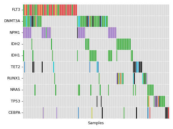
>>> vf.plot_comparison(a, b, c)
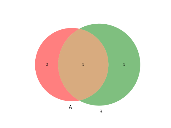
- plot_hist_format(k, af=None, group_col=None, group_order=None, kde=True, ax=None, figsize=None, **kwargs)[source]
Create a histogram showing the distribution of data for the specified FORMAT key.
- Parameters:
k (str) – One of the special FORMAT keys as defined in
VcfFrame.extract_format().af (common.AnnFrame) – AnnFrame containing sample annotation data.
group_col (list, optional) – AnnFrame column containing sample group information.
group_order (list, optional) – List of sample group names.
kde (bool, default: True) – Compute a kernel density estimate to smooth the distribution.
ax (matplotlib.axes.Axes, optional) – Pre-existing axes for the plot. Otherwise, crete a new one.
figsize (tuple, optional) – Width, height in inches. Format: (float, float).
kwargs – Other keyword arguments will be passed down to
seaborn.histplot().
- Returns:
The matplotlib axes containing the plot.
- Return type:
matplotlib.axes.Axes
Examples
Below is a simple example:
>>> from fuc import common, pyvcf >>> common.load_dataset('pyvcf') >>> vcf_file = '~/fuc-data/pyvcf/normal-tumor.vcf' >>> vf = pyvcf.VcfFrame.from_file(vcf_file) >>> vf.plot_hist_format('#DP')
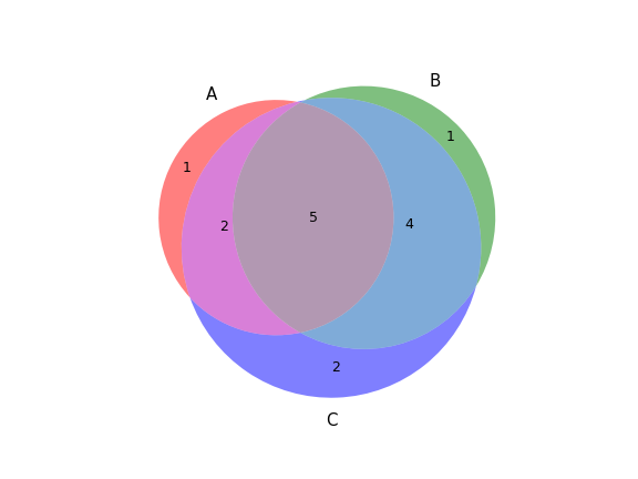
We can draw multiple histograms with hue mapping:
>>> annot_file = '~/fuc-data/pyvcf/normal-tumor-annot.tsv' >>> af = common.AnnFrame.from_file(annot_file, sample_col='Sample') >>> vf.plot_hist_format('#DP', af=af, group_col='Tissue')
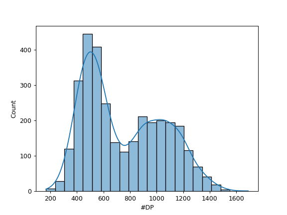
We can show AF instead of DP:
>>> vf.plot_hist_format('#AD_FRAC_REF')
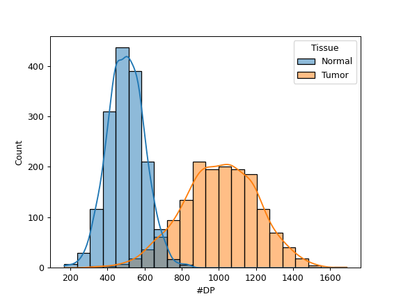
- plot_hist_info(k, kde=True, ax=None, figsize=None, **kwargs)[source]
Create a histogram showing the distribution of data for the specified INFO key.
- Parameters:
k (str) – One of the special INFO keys as defined in
VcfFrame.extract_info().kde (bool, default: True) – Compute a kernel density estimate to smooth the distribution.
ax (matplotlib.axes.Axes, optional) – Pre-existing axes for the plot. Otherwise, crete a new one.
figsize (tuple, optional) – Width, height in inches. Format: (float, float).
kwargs – Other keyword arguments will be passed down to
seaborn.histplot().
- Returns:
The matplotlib axes containing the plot.
- Return type:
matplotlib.axes.Axes
Examples
Below is a simple example:
>>> from fuc import common, pyvcf >>> common.load_dataset('pyvcf') >>> vcf_file = '~/fuc-data/pyvcf/getrm-cyp2d6-vdr.vcf' >>> vf = pyvcf.VcfFrame.from_file(vcf_file) >>> vf.plot_hist_info('#AC')
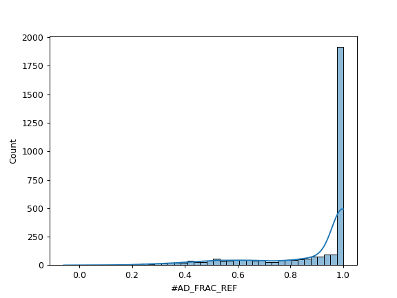
We can show AF instead of AC:
>>> vf.plot_hist_info('#AF')

- plot_rainfall(sample, palette=None, ax=None, figsize=None, legend='auto', **kwargs)[source]
Create a rainfall plot visualizing inter-variant distance on a linear genomic scale for single sample.
Under the hood, this method simply converts the VcfFrame to the
fuc.api.pymaf.MafFrameclass and then applies thefuc.api.pymaf.MafFrame.plot_rainfall()method.- Parameters:
sample (str) – Name of the sample.
palette (str, optional) – Name of the seaborn palette. See the Control plot colors tutorial for details.
ax (matplotlib.axes.Axes, optional) – Pre-existing axes for the plot. Otherwise, crete a new one.
figsize (tuple, optional) – Width, height in inches. Format: (float, float).
kwargs – Other keyword arguments will be passed down to
seaborn.scatterplot().
- Returns:
The matplotlib axes containing the plot.
- Return type:
matplotlib.axes.Axes
See also
fuc.api.pymaf.MafFrame.plot_rainfallSimilar method for the
fuc.api.pymaf.MafFrame()class.
Examples
>>> import matplotlib.pyplot as plt >>> import seaborn as sns >>> from fuc import common, pyvcf >>> common.load_dataset('brca') >>> vcf_file = '~/fuc-data/brca/brca.vcf' >>> vf = pyvcf.VcfFrame.from_file(vcf_file) >>> vf.plot_rainfall('TCGA-A8-A08B', ... figsize=(14, 7), ... palette=sns.color_palette('Set2')[:6]) >>> plt.tight_layout()
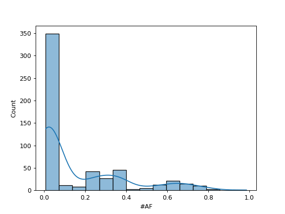
- plot_region(sample, k='#DP', color=None, region=None, label=None, ax=None, figsize=None, **kwargs)[source]
Create a scatter plot showing read depth profile of a sample for the specified region.
- Parameters:
sample (str or int) – Name or index of target sample.
k (str, default: ‘#DP’) – Genotype key to use for extracting data:
‘#DP’: Return read depth.
‘#AD_REF’: Return REF allele depth.
‘#AD_ALT’: Return ALT allele depth.
‘#AD_FRAC_REF’: Return REF allele fraction.
‘#AD_FRAC_ALT’: Return ALT allele fraction.
color (str, optional) – Marker color.
region (str, optional) – Target region (‘chrom:start-end’).
label (str, optional) – Label to use for the data points.
ax (matplotlib.axes.Axes, optional) – Pre-existing axes for the plot. Otherwise, crete a new one.
figsize (tuple, optional) – Width, height in inches. Format: (float, float).
kwargs – Other keyword arguments will be passed down to
matplotlib.axes.Axes.scatter().
- Returns:
The matplotlib axes containing the plot.
- Return type:
matplotlib.axes.Axes
Examples
Below is a simple example:
>>> from fuc import pyvcf, common >>> import matplotlib.pyplot as plt >>> common.load_dataset('pyvcf') >>> vcf_file = '~/fuc-data/pyvcf/getrm-cyp2d6-vdr.vcf' >>> vf = pyvcf.VcfFrame.from_file(vcf_file) >>> vf.plot_region('NA18973') >>> plt.tight_layout()
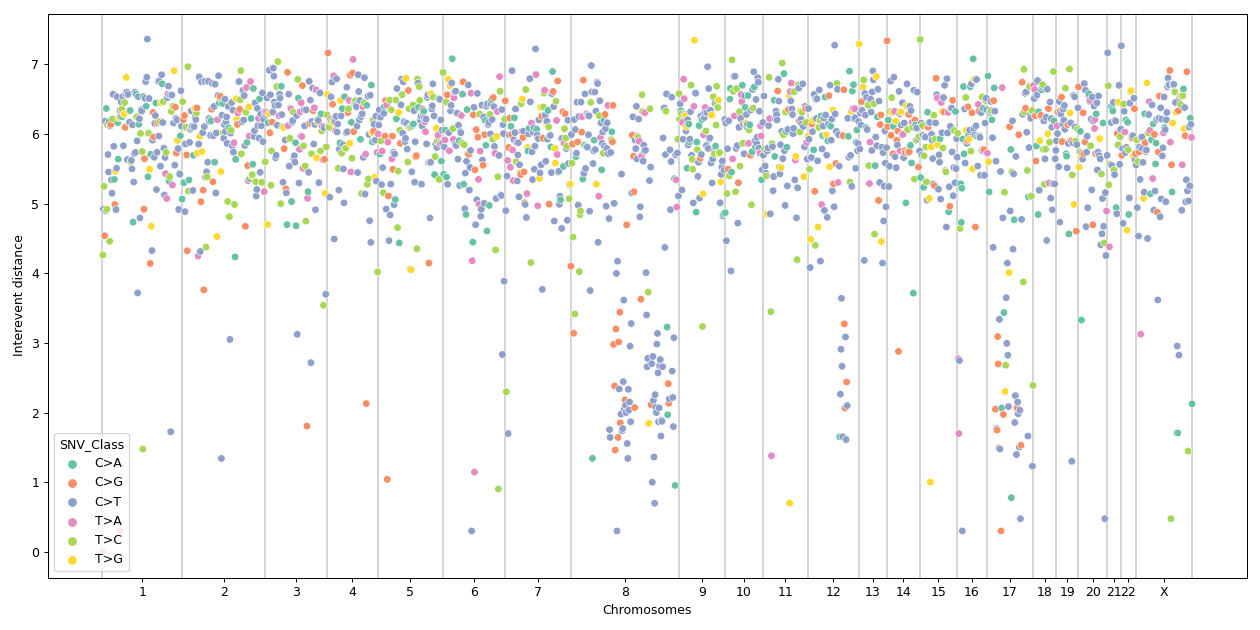
We can display allele fraction of REF and ALT instead of DP:
>>> ax = vf.plot_region('NA18973', k='#AD_FRAC_REF', label='REF') >>> vf.plot_region('NA18973', k='#AD_FRAC_ALT', label='ALT', ax=ax) >>> plt.tight_layout()
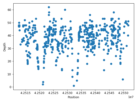
- plot_regplot_tmb(a, b, ax=None, figsize=None, **kwargs)[source]
Create a scatter plot with a linear regression model fit visualizing correlation between TMB in two sample groups.
The method will automatically calculate and print summary statistics including R-squared and p-value.
- Parameters:
a, b (array-like) – Lists of sample names. The lists must have the same shape.
ax (matplotlib.axes.Axes, optional) – Pre-existing axes for the plot. Otherwise, crete a new one.
figsize (tuple, optional) – Width, height in inches. Format: (float, float).
kwargs – Other keyword arguments will be passed down to
seaborn.regplot().
- Returns:
The matplotlib axes containing the plot.
- Return type:
matplotlib.axes.Axes
See also
fuc.api.pymaf.MafFrame.plot_regplot_tmbSimilar method for the
fuc.api.pymaf.MafFrame()class.
Examples
>>> from fuc import common, pyvcf >>> common.load_dataset('pyvcf') >>> vcf_file = '~/fuc-data/pyvcf/normal-tumor.vcf' >>> annot_file = '~/fuc-data/pyvcf/normal-tumor-annot.tsv' >>> vf = pyvcf.VcfFrame.from_file(vcf_file) >>> af = common.AnnFrame.from_file(annot_file, sample_col='Sample') >>> normal = af.df[af.df.Tissue == 'Normal'].index >>> normal.name = 'Normal' >>> tumor = af.df[af.df.Tissue == 'Tumor'].index >>> tumor.name = 'Tumor' >>> vf.plot_regplot_tmb(normal, tumor) Results for B ~ A: R^2 = 0.01 P = 7.17e-01 >>> plt.tight_layout()
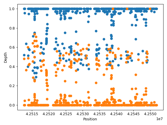
- plot_snvclsc(af=None, group_col=None, group_order=None, palette=None, flip=False, ax=None, figsize=None, **kwargs)[source]
Create a bar plot summarizing the count distrubtions of the six SNV classes for all samples.
A grouped bar plot can be created with
group_col(requires an AnnFrame).Under the hood, this method simply converts the VcfFrame to the
fuc.api.pymaf.MafFrameclass and then applies thefuc.api.pymaf.MafFrame.plot_snvclsc()method.- Parameters:
af (AnnFrame, optional) – AnnFrame containing sample annotation data.
group_col (str, optional) – AnnFrame column containing sample group information.
group_order (list, optional) – List of sample group names.
palette (str, optional) – Name of the seaborn palette. See the Control plot colors tutorial for details.
flip (bool, default: False) – If True, flip the x and y axes.
ax (matplotlib.axes.Axes, optional) – Pre-existing axes for the plot. Otherwise, crete a new one.
figsize (tuple, optional) – Width, height in inches. Format: (float, float).
kwargs – Other keyword arguments will be passed down to
seaborn.barplot().
- Returns:
The matplotlib axes containing the plot.
- Return type:
matplotlib.axes.Axes
See also
fuc.api.pymaf.MafFrame.plot_snvclscSimilar method for the
fuc.api.pymaf.MafFrame()class.
Examples
Below is a simple example:
>>> import matplotlib.pyplot as plt >>> import seaborn as sns >>> from fuc import common, pyvcf >>> common.load_dataset('tcga-laml') >>> vcf_file = '~/fuc-data/tcga-laml/tcga_laml.vcf' >>> vf = pyvcf.VcfFrame.from_file(vcf_file) >>> vf.plot_snvclsc(palette=sns.color_palette('Pastel1')) >>> plt.tight_layout()
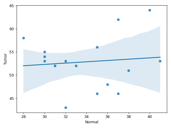
We can create a grouped bar plot based on FAB classification:
>>> annot_file = '~/fuc-data/tcga-laml/tcga_laml_annot.tsv' >>> af = common.AnnFrame.from_file(annot_file, sample_col=0) >>> vf.plot_snvclsc(af=af, ... group_col='FAB_classification', ... group_order=['M0', 'M1', 'M2']) >>> plt.tight_layout()
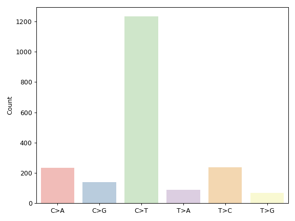
- plot_snvclsp(af=None, group_col=None, group_order=None, palette=None, flip=False, ax=None, figsize=None, **kwargs)[source]
Create a box plot summarizing the proportion distrubtions of the six SNV classes for all sample.
Under the hood, this method simply converts the VcfFrame to the
fuc.api.pymaf.MafFrameclass and then applies thefuc.api.pymaf.MafFrame.plot_snvclsp()method.- Parameters:
af (AnnFrame, optional) – AnnFrame containing sample annotation data.
group_col (str, optional) – AnnFrame column containing sample group information.
group_order (list, optional) – List of sample group names.
palette (str, optional) – Name of the seaborn palette. See the Control plot colors tutorial for details.
flip (bool, default: False) – If True, flip the x and y axes.
ax (matplotlib.axes.Axes, optional) – Pre-existing axes for the plot. Otherwise, crete a new one.
figsize (tuple, optional) – Width, height in inches. Format: (float, float).
kwargs – Other keyword arguments will be passed down to
seaborn.boxplot().
- Returns:
The matplotlib axes containing the plot.
- Return type:
matplotlib.axes.Axes
See also
fuc.api.pymaf.MafFrame.plot_snvclspSimilar method for the
fuc.api.pymaf.MafFrame()class.
Examples
Below is a simple example:
>>> import matplotlib.pyplot as plt >>> import seaborn as sns >>> from fuc import common, pyvcf >>> common.load_dataset('tcga-laml') >>> vcf_file = '~/fuc-data/tcga-laml/tcga_laml.vcf' >>> vf = pyvcf.VcfFrame.from_file(vcf_file) >>> vf.plot_snvclsp(palette=sns.color_palette('Pastel1')) >>> plt.tight_layout()
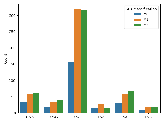
We can create a grouped bar plot based on FAB classification:
>>> annot_file = '~/fuc-data/tcga-laml/tcga_laml_annot.tsv' >>> af = common.AnnFrame.from_file(annot_file, sample_col=0) >>> vf.plot_snvclsp(af=af, ... group_col='FAB_classification', ... group_order=['M0', 'M1', 'M2']) >>> plt.tight_layout()
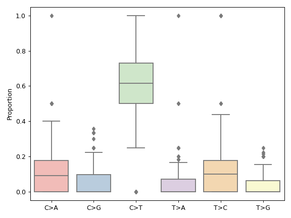
- plot_snvclss(color=None, colormap=None, width=0.8, legend=True, flip=False, ax=None, figsize=None, **kwargs)[source]
Create a bar plot showing the proportions of the six SNV classes for individual samples.
Under the hood, this method simply converts the VcfFrame to the
fuc.api.pymaf.MafFrameclass and then applies thefuc.api.pymaf.MafFrame.plot_snvclss()method.- Parameters:
color (list, optional) – List of color tuples. See the Control plot colors tutorial for details.
colormap (str or matplotlib colormap object, optional) – Colormap to select colors from. See the Control plot colors tutorial for details.
width (float, default: 0.8) – The width of the bars.
legend (bool, default: True) – Place legend on axis subplots.
flip (bool, default: False) – If True, flip the x and y axes.
ax (matplotlib.axes.Axes, optional) – Pre-existing axes for the plot. Otherwise, crete a new one.
figsize (tuple, optional) – Width, height in inches. Format: (float, float).
kwargs – Other keyword arguments will be passed down to
pandas.DataFrame.plot.bar()orpandas.DataFrame.plot.barh().
- Returns:
The matplotlib axes containing the plot.
- Return type:
matplotlib.axes.Axes
See also
fuc.api.pymaf.MafFrame.plot_snvclssSimilar method for the
fuc.api.pymaf.MafFrame()class.
Examples
>>> import matplotlib.pyplot as plt >>> from fuc import common, pymaf >>> common.load_dataset('tcga-laml') >>> maf_file = '~/fuc-data/tcga-laml/tcga_laml.maf.gz' >>> mf = pymaf.MafFrame.from_file(maf_file) >>> ax = mf.plot_snvclss(width=1, color=plt.get_cmap('Pastel1').colors) >>> ax.legend(loc='upper right') >>> plt.tight_layout()
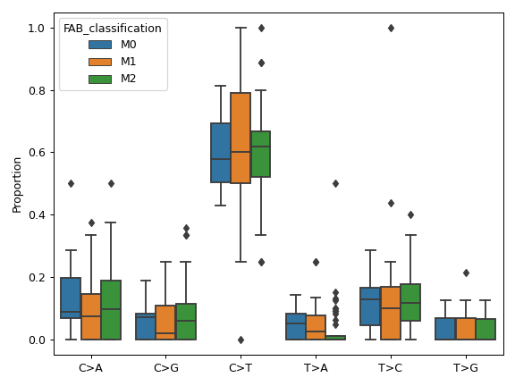
- plot_titv(af=None, group_col=None, group_order=None, flip=False, ax=None, figsize=None, **kwargs)[source]
Create a box plot showing the Ti/Tv proportions of samples.
Under the hood, this method simply converts the VcfFrame to the
pymaf.MafFrameclass and then applies thepymaf.MafFrame.plot_titv()method.- Parameters:
af (AnnFrame, optional) – AnnFrame containing sample annotation data.
group_col (str, optional) – AnnFrame column containing sample group information.
group_order (list, optional) – List of sample group names.
flip (bool, default: False) – If True, flip the x and y axes.
ax (matplotlib.axes.Axes, optional) – Pre-existing axes for the plot. Otherwise, crete a new one.
figsize (tuple, optional) – Width, height in inches. Format: (float, float).
kwargs – Other keyword arguments will be passed down to
seaborn.boxplot().
- Returns:
The matplotlib axes containing the plot.
- Return type:
matplotlib.axes.Axes
See also
fuc.api.pymaf.MafFrame.plot_titvSimilar method for the
fuc.api.pymaf.MafFrameclass.
Examples
Below is a simple example:
>>> import matplotlib.pyplot as plt >>> from fuc import common, pyvcf >>> common.load_dataset('tcga-laml') >>> vcf_file = '~/fuc-data/tcga-laml/tcga_laml.vcf' >>> vf = pyvcf.VcfFrame.from_file(vcf_file) >>> vf.plot_titv() >>> plt.tight_layout()
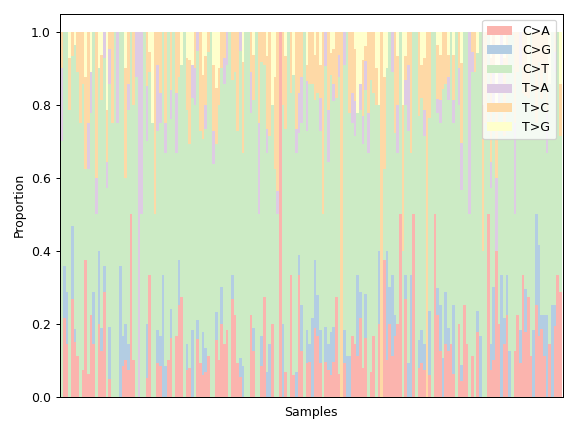
We can create a grouped bar plot based on FAB classification:
>>> annot_file = '~/fuc-data/tcga-laml/tcga_laml_annot.tsv' >>> af = common.AnnFrame.from_file(annot_file, sample_col=0) >>> vf.plot_titv(af=af, ... group_col='FAB_classification', ... group_order=['M0', 'M1', 'M2']) >>> plt.tight_layout()
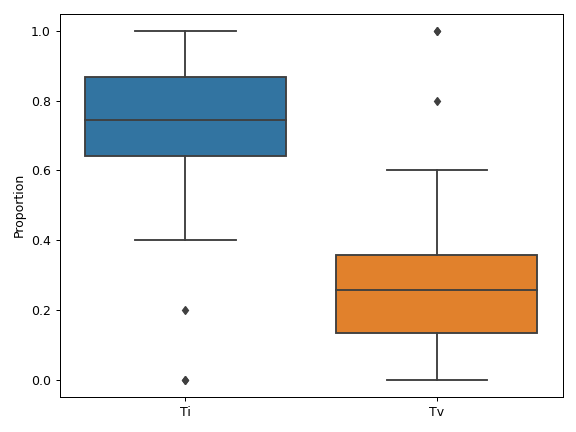
- plot_tmb(af=None, group_col=None, group_order=None, kde=True, ax=None, figsize=None, **kwargs)[source]
Create a histogram showing TMB distribution.
- Parameters:
af (common.AnnFrame) – AnnFrame containing sample annotation data (requires
hue).group_col (str, optional) – AnnFrame column containing sample group information.
group_order (list, optional) – List of sample group names.
kde (bool, default: True) – Compute a kernel density estimate to smooth the distribution.
ax (matplotlib.axes.Axes, optional) – Pre-existing axes for the plot. Otherwise, crete a new one.
figsize (tuple, optional) – Width, height in inches. Format: (float, float).
kwargs – Other keyword arguments will be passed down to
seaborn.histplot().
- Returns:
The matplotlib axes containing the plot.
- Return type:
matplotlib.axes.Axes
Examples
Below is a simple example:
>>> from fuc import common, pyvcf >>> common.load_dataset('pyvcf') >>> vcf_file = '~/fuc-data/pyvcf/normal-tumor.vcf' >>> vf = pyvcf.VcfFrame.from_file(vcf_file) >>> vf.plot_tmb()
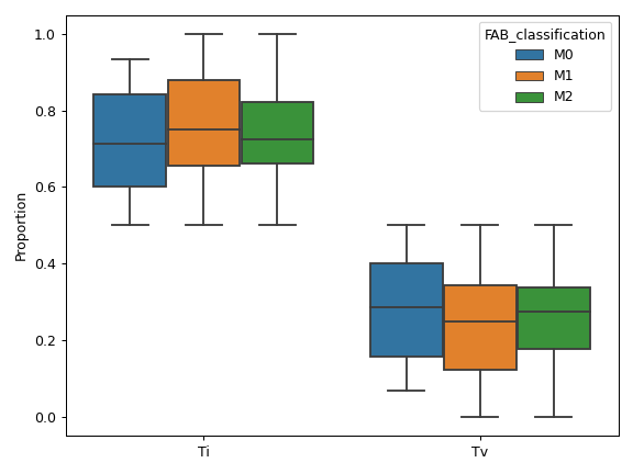
We can draw multiple histograms with hue mapping:
>>> annot_file = '~/fuc-data/pyvcf/normal-tumor-annot.tsv' >>> af = common.AnnFrame.from_file(annot_file, sample_col='Sample') >>> vf.plot_tmb(af=af, group_col='Tissue')
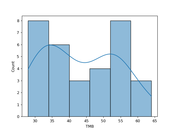
- pseudophase()[source]
Pseudophase VcfFrame.
- Returns:
Pseudophased VcfFrame.
- Return type:
Examples
>>> from fuc import pyvcf >>> data = { ... 'CHROM': ['chr1', 'chr2'], ... 'POS': [100, 101], ... 'ID': ['.', '.'], ... 'REF': ['G', 'T'], ... 'ALT': ['A', 'C'], ... 'QUAL': ['.', '.'], ... 'FILTER': ['.', '.'], ... 'INFO': ['.', '.'], ... 'FORMAT': ['GT', 'GT'], ... 'A': ['0/1', '1/1'] ... } >>> vf = pyvcf.VcfFrame.from_dict([], data) >>> vf.df CHROM POS ID REF ALT QUAL FILTER INFO FORMAT A 0 chr1 100 . G A . . . GT 0/1 1 chr2 101 . T C . . . GT 1/1 >>> vf.pseudophase().df CHROM POS ID REF ALT QUAL FILTER INFO FORMAT A 0 chr1 100 . G A . . . GT 0|1 1 chr2 101 . T C . . . GT 1|1
- rename(names, indicies=None)[source]
Rename the samples.
- Parameters:
names (dict or list) – Dict of old names to new names or list of new names.
indicies (list or tuple, optional) – List of 0-based sample indicies. Alternatively, a tuple (int, int) can be used to specify an index range.
- Returns:
Updated VcfFrame.
- Return type:
Examples
>>> from fuc import pyvcf >>> data = { ... 'CHROM': ['chr1', 'chr2'], ... 'POS': [100, 101], ... 'ID': ['.', '.'], ... 'REF': ['G', 'T'], ... 'ALT': ['A', 'C'], ... 'QUAL': ['.', '.'], ... 'FILTER': ['.', '.'], ... 'INFO': ['.', '.'], ... 'FORMAT': ['GT', 'GT'], ... 'A': ['0/1', '0/1'], ... 'B': ['0/1', '0/1'], ... 'C': ['0/1', '0/1'], ... 'D': ['0/1', '0/1'], ... } >>> vf = pyvcf.VcfFrame.from_dict([], data) >>> vf.df CHROM POS ID REF ALT QUAL FILTER INFO FORMAT A B C D 0 chr1 100 . G A . . . GT 0/1 0/1 0/1 0/1 1 chr2 101 . T C . . . GT 0/1 0/1 0/1 0/1 >>> vf.rename(['1', '2', '3', '4']).df CHROM POS ID REF ALT QUAL FILTER INFO FORMAT 1 2 3 4 0 chr1 100 . G A . . . GT 0/1 0/1 0/1 0/1 1 chr2 101 . T C . . . GT 0/1 0/1 0/1 0/1 >>> vf.rename({'B': '2', 'C': '3'}).df CHROM POS ID REF ALT QUAL FILTER INFO FORMAT A 2 3 D 0 chr1 100 . G A . . . GT 0/1 0/1 0/1 0/1 1 chr2 101 . T C . . . GT 0/1 0/1 0/1 0/1 >>> vf.rename(['2', '4'], indicies=[1, 3]).df CHROM POS ID REF ALT QUAL FILTER INFO FORMAT A 2 C 4 0 chr1 100 . G A . . . GT 0/1 0/1 0/1 0/1 1 chr2 101 . T C . . . GT 0/1 0/1 0/1 0/1 >>> vf.rename(['2', '3'], indicies=(1, 3)).df CHROM POS ID REF ALT QUAL FILTER INFO FORMAT A 2 3 D 0 chr1 100 . G A . . . GT 0/1 0/1 0/1 0/1 1 chr2 101 . T C . . . GT 0/1 0/1 0/1 0/1
- property samples
List of sample names.
- Type:
list
- property shape
Dimensionality of VcfFrame (variants, samples).
- Type:
tuple
- property sites_only
Whether the VCF is sites-only.
- Type:
bool
- slice(region)[source]
Slice VcfFrame for specified region.
- Parameters:
region (str) – Region to slice (‘chrom:start-end’). The ‘chr’ string will be handled automatically. For example, ‘chr1’ and ‘1’ will have the same effect in slicing.
- Returns:
Sliced VcfFrame.
- Return type:
Examples
Assume we have following data:
>>> from fuc import pyvcf >>> data = { ... 'CHROM': ['chr1', 'chr1', 'chr1', 'chr2'], ... 'POS': [100, 205, 297, 101], ... 'ID': ['.', '.', '.', '.'], ... 'REF': ['G', 'T', 'A', 'C'], ... 'ALT': ['A', 'C', 'T', 'A'], ... 'QUAL': ['.', '.', '.', '.'], ... 'FILTER': ['.', '.', '.', '.'], ... 'INFO': ['.', '.', '.', '.'], ... 'FORMAT': ['GT', 'GT', 'GT', 'GT'], ... 'A': ['0/1', '1/1', '0/0', '0/0'], ... 'B': ['0/0', '0/0', '0/1', '0/1'], ... } >>> vf = pyvcf.VcfFrame.from_dict([], data) >>> vf.df CHROM POS ID REF ALT QUAL FILTER INFO FORMAT A B 0 chr1 100 . G A . . . GT 0/1 0/0 1 chr1 205 . T C . . . GT 1/1 0/0 2 chr1 297 . A T . . . GT 0/0 0/1 3 chr2 101 . C A . . . GT 0/0 0/1
We can specify a full region:
>>> vf.slice('chr1:101-300').df CHROM POS ID REF ALT QUAL FILTER INFO FORMAT A B 0 chr1 205 . T C . . . GT 1/1 0/0 1 chr1 297 . A T . . . GT 0/0 0/1
We can specify a region without the ‘chr’ string:
>>> vf.slice('1:101-300').df CHROM POS ID REF ALT QUAL FILTER INFO FORMAT A B 0 chr1 205 . T C . . . GT 1/1 0/0 1 chr1 297 . A T . . . GT 0/0 0/1
We can specify the contig only:
>>> vf.slice('chr1').df CHROM POS ID REF ALT QUAL FILTER INFO FORMAT A B 0 chr1 100 . G A . . . GT 0/1 0/0 1 chr1 205 . T C . . . GT 1/1 0/0 2 chr1 297 . A T . . . GT 0/0 0/1
We can omit the start position:
>>> vf.slice('chr1:-296').df CHROM POS ID REF ALT QUAL FILTER INFO FORMAT A B 0 chr1 100 . G A . . . GT 0/1 0/0 1 chr1 205 . T C . . . GT 1/1 0/0
We can omit the end position as well:
>>> vf.slice('chr1:101').df CHROM POS ID REF ALT QUAL FILTER INFO FORMAT A B 0 chr1 205 . T C . . . GT 1/1 0/0 1 chr1 297 . A T . . . GT 0/0 0/1
You can also omit the end position this way:
>>> vf.slice('chr1:101-').df CHROM POS ID REF ALT QUAL FILTER INFO FORMAT A B 0 chr1 205 . T C . . . GT 1/1 0/0 1 chr1 297 . A T . . . GT 0/0 0/1
- sort()[source]
Sort the VcfFrame by chromosome and position.
- Returns:
Sorted VcfFrame.
- Return type:
Examples
Assume we have the following data:
>>> from fuc import pyvcf >>> data = { ... 'CHROM': ['chr10', 'chr2', 'chr1', 'chr2'], ... 'POS': [100, 101, 102, 90], ... 'ID': ['.', '.', '.', '.'], ... 'REF': ['G', 'T', 'T', 'A'], ... 'ALT': ['A', 'C', 'A', 'T'], ... 'QUAL': ['.', '.', '.', '.'], ... 'FILTER': ['.', '.', '.', '.'], ... 'INFO': ['.', '.', '.', '.'], ... 'FORMAT': ['GT:DP', 'GT:DP', 'GT:DP', 'GT:DP'], ... 'Steven': ['./.:.', '0/0:29', '0/0:28', '0/1:17'] ... } >>> vf = pyvcf.VcfFrame.from_dict([], data) >>> vf.df CHROM POS ID REF ALT QUAL FILTER INFO FORMAT Steven 0 chr10 100 . G A . . . GT:DP ./.:. 1 chr2 101 . T C . . . GT:DP 0/0:29 2 chr1 102 . T A . . . GT:DP 0/0:28 3 chr2 90 . A T . . . GT:DP 0/1:17
We can sort the VcfFrame by:
>>> vf.sort().df CHROM POS ID REF ALT QUAL FILTER INFO FORMAT Steven 0 chr1 102 . T A . . . GT:DP 0/0:28 1 chr2 90 . A T . . . GT:DP 0/1:17 2 chr2 101 . T C . . . GT:DP 0/0:29 3 chr10 100 . G A . . . GT:DP ./.:.
- strip(format='GT', metadata=False)[source]
Remove any unnecessary data.
- Parameters:
format (str, default: ‘GT’) – FORMAT keys to retain (e.g. ‘GT:AD:DP’).
metadata (bool, default: False) – If True, keep the metadata.
- Returns:
Stripped VcfFrame.
- Return type:
Examples
>>> from fuc import pyvcf >>> data = { ... 'CHROM': ['chr1', 'chr1', 'chr1'], ... 'POS': [100, 101, 102], ... 'ID': ['.', '.', '.'], ... 'REF': ['G', 'T', 'A'], ... 'ALT': ['A', 'C', 'T'], ... 'QUAL': ['.', '.', '.'], ... 'FILTER': ['.', '.', '.'], ... 'INFO': ['.', '.', '.'], ... 'FORMAT': ['GT:DP:AD', 'GT:DP:AD', 'GT'], ... 'A': ['0/1:30:15,15', '1/1:28:0,28', '0/1'] ... } >>> vf = pyvcf.VcfFrame.from_dict([], data) >>> vf.df CHROM POS ID REF ALT QUAL FILTER INFO FORMAT A 0 chr1 100 . G A . . . GT:DP:AD 0/1:30:15,15 1 chr1 101 . T C . . . GT:DP:AD 1/1:28:0,28 2 chr1 102 . A T . . . GT 0/1 >>> vf.strip('GT:DP').df CHROM POS ID REF ALT QUAL FILTER INFO FORMAT A 0 chr1 100 . G A . . . GT:DP 0/1:30 1 chr1 101 . T C . . . GT:DP 1/1:28 2 chr1 102 . A T . . . GT:DP 0/1:.
- subset(samples, exclude=False)[source]
Subset VcfFrame for specified samples.
- Parameters:
samples (str or list) – Sample name or list of names (the order matters).
exclude (bool, default: False) – If True, exclude specified samples.
- Returns:
Subsetted VcfFrame.
- Return type:
Examples
Assume we have the following data:
>>> from fuc import pyvcf >>> data = { ... 'CHROM': ['chr1', 'chr1'], ... 'POS': [100, 101], ... 'ID': ['.', '.'], ... 'REF': ['G', 'T'], ... 'ALT': ['A', 'C'], ... 'QUAL': ['.', '.'], ... 'FILTER': ['.', '.'], ... 'INFO': ['.', '.'], ... 'FORMAT': ['GT', 'GT'], ... 'A': ['0/1', '0/1'], ... 'B': ['0/0', '0/1'], ... 'C': ['0/0', '0/0'], ... 'D': ['0/1', '0/0'], ... } >>> vf = pyvcf.VcfFrame.from_dict([], data) >>> vf.df CHROM POS ID REF ALT QUAL FILTER INFO FORMAT A B C D 0 chr1 100 . G A . . . GT 0/1 0/0 0/0 0/1 1 chr1 101 . T C . . . GT 0/1 0/1 0/0 0/0
We can subset the VcfFrame for the samples A and B:
>>> vf.subset(['A', 'B']).df CHROM POS ID REF ALT QUAL FILTER INFO FORMAT A B 0 chr1 100 . G A . . . GT 0/1 0/0 1 chr1 101 . T C . . . GT 0/1 0/1
Alternatively, we can exclude those samples:
>>> vf.subset(['A', 'B'], exclude=True).df CHROM POS ID REF ALT QUAL FILTER INFO FORMAT C D 0 chr1 100 . G A . . . GT 0/0 0/1 1 chr1 101 . T C . . . GT 0/0 0/0
- subtract(a, b)[source]
Subtract genotype data between two samples (A, B).
This method can be especially useful when you want to distinguish between somatic and germline variants for an individual. See examples below for more details.
- Parameters:
a, b (str or int) – Name or index of Samples A and B.
- Returns:
Resulting VCF column.
- Return type:
pandas.Series
See also
VcfFrame.combineCombine genotype data from two samples (A, B).
Examples
Assume we have following data for a cancer patient:
>>> from fuc import pyvcf >>> data = { ... 'CHROM': ['chr1', 'chr1', 'chr1', 'chr1', 'chr1'], ... 'POS': [100, 101, 102, 103, 104], ... 'ID': ['rs1', 'rs2', 'rs3', 'rs4', 'rs5'], ... 'REF': ['G', 'T', 'C', 'A', 'G'], ... 'ALT': ['A', 'G', 'T', 'C', 'C'], ... 'QUAL': ['.', '.', '.', '.', '.'], ... 'FILTER': ['.', '.', '.', '.', '.'], ... 'INFO': ['.', '.', '.', '.', '.'], ... 'FORMAT': ['GT', 'GT', 'GT', 'GT', 'GT'], ... 'Tissue': ['./.', '0/1', '0/1', '0/0', '0/1'], ... 'Blood': ['0/1', '0/1', './.', '0/1', '0/0'], ... } >>> vf = pyvcf.VcfFrame.from_dict([], data) >>> vf.df CHROM POS ID REF ALT QUAL FILTER INFO FORMAT Tissue Blood 0 chr1 100 rs1 G A . . . GT ./. 0/1 1 chr1 101 rs2 T G . . . GT 0/1 0/1 2 chr1 102 rs3 C T . . . GT 0/1 ./. 3 chr1 103 rs4 A C . . . GT 0/0 0/1 4 chr1 104 rs5 G C . . . GT 0/1 0/0
We can compare genotype data between ‘Tissue’ and ‘Blood’ to identify somatic variants (i.e. rs3 and rs5; rs2 is most likely germline):
>>> vf.df['Somatic'] = vf.subtract('Tissue', 'Blood') >>> vf.df CHROM POS ID REF ALT QUAL FILTER INFO FORMAT Tissue Blood Somatic 0 chr1 100 rs1 G A . . . GT ./. 0/1 ./. 1 chr1 101 rs2 T G . . . GT 0/1 0/1 ./. 2 chr1 102 rs3 C T . . . GT 0/1 ./. 0/1 3 chr1 103 rs4 A C . . . GT 0/0 0/1 0/0 4 chr1 104 rs5 G C . . . GT 0/1 0/0 0/1
- to_bed()[source]
Convert VcfFrame to BedFrame.
- Returns:
BedFrame obejct.
- Return type:
Examples
Assume we have the following data:
>>> from fuc import pyvcf >>> data = { ... 'CHROM': ['chr1', 'chr1', 'chr1', 'chr1', 'chr1'], ... 'POS': [100, 101, 102, 103, 104], ... 'ID': ['.', '.', '.', '.', '.'], ... 'REF': ['A', 'A', 'C', 'C', 'ACGT'], ... 'ALT': ['C', 'T,G', 'G', 'A,G,CT', 'A'], ... 'QUAL': ['.', '.', '.', '.', '.'], ... 'FILTER': ['.', '.', '.', '.', '.'], ... 'INFO': ['.', '.', '.', '.', '.'], ... 'FORMAT': ['GT:DP', 'GT:DP', 'GT:DP', 'GT:DP', 'GT:DP'], ... 'Steven': ['0/1:32', './.:.', '0/1:27', '0/2:34', '0/0:31'], ... 'Sara': ['0/0:28', '1/2:30', '1/1:29', '1/2:38', '0/1:27'], ... } >>> vf = pyvcf.VcfFrame.from_dict([], data) >>> vf.df CHROM POS ID REF ALT QUAL FILTER INFO FORMAT Steven Sara 0 chr1 100 . A C . . . GT:DP 0/1:32 0/0:28 1 chr1 101 . A T,G . . . GT:DP ./.:. 1/2:30 2 chr1 102 . C G . . . GT:DP 0/1:27 1/1:29 3 chr1 103 . C A,G,CT . . . GT:DP 0/2:34 1/2:38 4 chr1 104 . ACGT A . . . GT:DP 0/0:31 0/1:27
We can construct BedFrame from the VcfFrame:
>>> bf = vf.to_bed() >>> bf.gr.df Chromosome Start End 0 chr1 100 100 1 chr1 101 101 2 chr1 102 102 3 chr1 103 103 4 chr1 103 104 5 chr1 105 107
- to_file(fn, compression=False)[source]
Write VcfFrame to a VCF file.
If the filename ends with ‘.gz’, the method will automatically use the BGZF compression when writing the file.
- Parameters:
fn (str) – VCF file path.
compression (bool, default: False) – If True, use the BGZF compression.
Examples
>>> from fuc import pyvcf >>> data = { ... 'CHROM': ['chr1', 'chr2'], ... 'POS': [100, 101], ... 'ID': ['.', '.'], ... 'REF': ['G', 'T'], ... 'ALT': ['A', 'C'], ... 'QUAL': ['.', '.'], ... 'FILTER': ['.', '.'], ... 'INFO': ['.', '.'], ... 'FORMAT': ['GT', 'GT'], ... 'Steven': ['0/1', '1/1'] ... } >>> vf = pyvcf.VcfFrame.from_dict(['##fileformat=VCFv4.3'], data) >>> vf.to_file('unzipped.vcf') >>> vf.to_file('zipped.vcf.gz') >>> vf.to_file('zipped.vcf.gz', compression=True)
- to_string()[source]
Render the VcfFrame to a console-friendly tabular output.
- Returns:
String representation of the VcfFrame.
- Return type:
str
Examples
>>> from fuc import pyvcf >>> data = { ... 'CHROM': ['chr1', 'chr1'], ... 'POS': [100, 101], ... 'ID': ['.', '.'], ... 'REF': ['G', 'T'], ... 'ALT': ['A', 'C'], ... 'QUAL': ['.', '.'], ... 'FILTER': ['.', '.'], ... 'INFO': ['.', '.'], ... 'FORMAT': ['GT', 'GT'], ... 'A': ['0/1', '0/1'] ... } >>> vf = pyvcf.VcfFrame.from_dict(['##fileformat=VCFv4.3'], data) >>> print(vf.to_string()) ##fileformat=VCFv4.3 #CHROM POS ID REF ALT QUAL FILTER INFO FORMAT A chr1 100 . G A . . . GT 0/1 chr1 101 . T C . . . GT 0/1
- to_variants()[source]
List unique variants in VcfFrame.
- Returns:
List of unique variants.
- Return type:
list
Examples
>>> from fuc import pyvcf >>> data = { ... 'CHROM': ['chr1', 'chr2'], ... 'POS': [100, 101], ... 'ID': ['.', '.'], ... 'REF': ['G', 'T'], ... 'ALT': ['A', 'A,C'], ... 'QUAL': ['.', '.'], ... 'FILTER': ['.', '.'], ... 'INFO': ['.', '.'], ... 'FORMAT': ['GT', 'GT'], ... 'A': ['0/1', '1/2'] ... } >>> vf = pyvcf.VcfFrame.from_dict([], data) >>> vf.variants() ['chr1-100-G-A', 'chr2-101-T-A', 'chr2-101-T-C']
- unphase()[source]
Unphase all the sample genotypes.
- Returns:
Unphased VcfFrame.
- Return type:
Examples
Assume we have the following data:
>>> from fuc import pyvcf >>> data = { ... 'CHROM': ['chr1', 'chr1', 'chr1', 'chr1'], ... 'POS': [100, 101, 102, 103], ... 'ID': ['.', '.', '.', '.'], ... 'REF': ['G', 'T', 'A', 'C'], ... 'ALT': ['A', 'C', 'T', 'A'], ... 'QUAL': ['.', '.', '.', '.'], ... 'FILTER': ['.', '.', '.', '.'], ... 'INFO': ['.', '.', '.', '.'], ... 'FORMAT': ['GT', 'GT', 'GT', 'GT'], ... 'Steven': ['1|0', './.', '0|1', '0/1'], ... } >>> vf = pyvcf.VcfFrame.from_dict([], data) >>> vf.df CHROM POS ID REF ALT QUAL FILTER INFO FORMAT Steven 0 chr1 100 . G A . . . GT 1|0 1 chr1 101 . T C . . . GT ./. 2 chr1 102 . A T . . . GT 0|1 3 chr1 103 . C A . . . GT 0/1
We can unphase the samples genotypes:
>>> vf.unphase().df CHROM POS ID REF ALT QUAL FILTER INFO FORMAT Steven 0 chr1 100 . G A . . . GT 0/1 1 chr1 101 . T C . . . GT ./. 2 chr1 102 . A T . . . GT 0/1 3 chr1 103 . C A . . . GT 0/1
- update_chr_prefix(mode='remove')[source]
Add or remove the (annoying) ‘chr’ string from the CHROM column.
- Parameters:
mode ({‘add’, ‘remove’}, default: ‘remove’) – Whether to add or remove the ‘chr’ string.
- Returns:
Updated VcfFrame.
- Return type:
Examples
>>> from fuc import pyvcf >>> data = { ... 'CHROM': ['chr1', 'chr1', '2', '2'], ... 'POS': [100, 101, 100, 101], ... 'ID': ['.', '.', '.', '.'], ... 'REF': ['G', 'T', 'T', 'C'], ... 'ALT': ['A', 'C', 'C', 'G'], ... 'QUAL': ['.', '.', '.', '.'], ... 'FILTER': ['.', '.', '.', '.'], ... 'INFO': ['.', '.', '.', '.'], ... 'FORMAT': ['GT', 'GT', 'GT', 'GT'], ... 'A': ['0/1', '0/1', '0/1', '0/1'] ... } >>> vf = pyvcf.VcfFrame.from_dict([], data) >>> vf.df CHROM POS ID REF ALT QUAL FILTER INFO FORMAT A 0 chr1 100 . G A . . . GT 0/1 1 chr1 101 . T C . . . GT 0/1 2 2 100 . T C . . . GT 0/1 3 2 101 . C G . . . GT 0/1 >>> vf.update_chr_prefix(mode='remove').df CHROM POS ID REF ALT QUAL FILTER INFO FORMAT A 0 1 100 . G A . . . GT 0/1 1 1 101 . T C . . . GT 0/1 2 2 100 . T C . . . GT 0/1 3 2 101 . C G . . . GT 0/1 >>> vf.update_chr_prefix(mode='add').df CHROM POS ID REF ALT QUAL FILTER INFO FORMAT A 0 chr1 100 . G A . . . GT 0/1 1 chr1 101 . T C . . . GT 0/1 2 chr2 100 . T C . . . GT 0/1 3 chr2 101 . C G . . . GT 0/1
- fuc.api.pyvcf.call(fasta, bams, regions=None, path=None, min_mq=1, max_depth=250, dir_path=None, gap_frac=0.002, group_samples=None)[source]
Call SNVs and indels from BAM files.
Under the hood, the method utilizes the bcftool program to call variants.
- Parameters:
fasta (str) – Reference FASTA file.
bams (str or list) – One or more input BAM files. Alternatively, you can provide a text file (.txt, .tsv, .csv, or .list) containing one BAM file per line.
regions (str, list, or pybed.BedFrame, optional) – By default (
regions=None), the method looks at each genomic position with coverage in BAM files, which can be excruciatingly slow for large files (e.g. whole genome sequencing). Therefore, use this argument to only call variants in given regions. Each region must have the format chrom:start-end and be a half-open interval with (start, end]. This means, for example, chr1:100-103 will extract positions 101, 102, and 103. Alternatively, you can provide a BED file (compressed or uncompressed) or apybed.BedFrameobject to specify regions. Note that the ‘chr’ prefix in contig names (e.g. ‘chr1’ vs. ‘1’) will be automatically added or removed as necessary to match the input VCF’s contig names.path (str, optional) – Output VCF file. Writes to stdout when
path='-'. If None is provided the result is returned as a string.min_mq (int, default: 1) – Minimum mapping quality for an alignment to be used.
max_depth (int, default: 250) – At a position, read maximally this number of reads per input file.
dir_path (str, optional) – By default, intermediate files (likelihoods.bcf, calls.bcf, and calls.normalized.bcf) will be stored in a temporary directory, which is automatically deleted after creating final VCF. If you provide a directory path, intermediate files will be stored there.
gap_frac (float, default: 0.002) – Minimum fraction of gapped reads for calling indels.
group_samples (str, optional) – By default, all samples are assumed to come from a single population. This option allows to group samples into populations and apply the HWE assumption within but not across the populations. To use this option, provide a tab-delimited text file with sample names in the first column and group names in the second column. If
group_samples='-'is given instead, no HWE assumption is made at all and single-sample calling is performed. Note that in low coverage data this inflates the rate of false positives. Therefore, make sure you know what you are doing.
- Returns:
VcfFrame object.
- Return type:
str
- fuc.api.pyvcf.gt_diploidize(g)[source]
For given genotype, return its diploid form.
This method will ignore diploid genotypes (e.g. 0/1) and is therefore only effective for haploid genotypes (e.g. genotypes from the X chromosome for males).
- Parameters:
g (str) – Sample genotype.
- Returns:
Diploid genotype.
- Return type:
bool
See also
VcfFrame.diploidizeDiploidize VcfFrame.
Examples
>>> from fuc import pyvcf >>> pyvcf.gt_diploidize('0') '0/0' >>> pyvcf.gt_diploidize('1') '0/1' >>> pyvcf.gt_diploidize('.') './.' >>> pyvcf.gt_diploidize('1:34') '0/1:34' >>> pyvcf.gt_diploidize('0/1:34') '0/1:34' >>> pyvcf.gt_diploidize('./.') './.'
- fuc.api.pyvcf.gt_hasvar(g)[source]
For given genotype, return True if it has variation.
- Parameters:
g (str) – Sample genotype.
- Returns:
True if genotype has variation.
- Return type:
bool
Examples
>>> from fuc import pyvcf >>> pyvcf.gt_hasvar('0') False >>> pyvcf.gt_hasvar('0/0') False >>> pyvcf.gt_hasvar('./.') False >>> pyvcf.gt_hasvar('1') True >>> pyvcf.gt_hasvar('0/1') True >>> pyvcf.gt_hasvar('1/2') True >>> pyvcf.gt_hasvar('1|0') True >>> pyvcf.gt_hasvar('1|2:21:6:23,27') True
- fuc.api.pyvcf.gt_het(g)[source]
For given genotype, return True if it is heterozygous.
- Parameters:
g (str) – Genotype call.
- Returns:
True if genotype is heterozygous.
- Return type:
bool
Examples
>>> from fuc import pyvcf >>> pyvcf.gt_het('0/1') True >>> pyvcf.gt_het('0/0') False >>> pyvcf.gt_het('0|0') False >>> pyvcf.gt_het('1|0') True
- fuc.api.pyvcf.gt_miss(g)[source]
For given genotype, return True if it has missing value.
- Parameters:
g (str) – Sample genotype.
- Returns:
True if genotype is missing.
- Return type:
bool
Examples
>>> from fuc import pyvcf >>> pyvcf.gt_miss('0') False >>> pyvcf.gt_miss('0/0') False >>> pyvcf.gt_miss('0/1') False >>> pyvcf.gt_miss('0|0:48:1:51,51') False >>> pyvcf.gt_miss('./.:.:.') True >>> pyvcf.gt_miss('.:.') True >>> pyvcf.gt_miss('.') True >>> pyvcf.gt_miss('./.:13,3:16:41:41,0,402') True
- fuc.api.pyvcf.gt_ploidy(g)[source]
For given genotype, return its ploidy number.
- Parameters:
g (str) – Sample genotype.
- Returns:
Ploidy number.
- Return type:
int
Examples
>>> from fuc import pyvcf >>> pyvcf.gt_ploidy('1') 1 >>> pyvcf.gt_ploidy('.') 1 >>> pyvcf.gt_ploidy('0/1') 2 >>> pyvcf.gt_ploidy('./.') 2 >>> pyvcf.gt_ploidy('0|1') 2 >>> pyvcf.gt_ploidy('1|0|1') 3 >>> pyvcf.gt_ploidy('0/./1/1') 4
- fuc.api.pyvcf.gt_polyp(g)[source]
For given genotype, return True if it is polyploid.
- Parameters:
g (str) – Sample genotype.
- Returns:
True if genotype is polyploid.
- Return type:
bool
Examples
>>> from fuc import pyvcf >>> pyvcf.gt_polyp('1') False >>> pyvcf.gt_polyp('0/1') False >>> pyvcf.gt_polyp('0/1/1') True >>> pyvcf.gt_polyp('1|0|1') True >>> pyvcf.gt_polyp('0/./1/1') True
- fuc.api.pyvcf.gt_pseudophase(g)[source]
For given genotype, return its pseudophased form.
- Parameters:
g (str) – Genotype call.
- Returns:
Pseudophased genotype call.
- Return type:
str
Examples
>>> from fuc import pyvcf >>> pyvcf.gt_pseudophase('0/1') '0|1' >>> pyvcf.gt_pseudophase('0/0:34:10,24') '0|0:34:10,24'
- fuc.api.pyvcf.gt_unphase(g)[source]
For given genotype, return its unphased form.
- Parameters:
g (str) – Sample genotype.
- Returns:
Unphased genotype.
- Return type:
str
Examples
>>> from fuc import pyvcf >>> pyvcf.gt_unphase('1') '1' >>> pyvcf.gt_unphase('0/0') '0/0' >>> pyvcf.gt_unphase('0/1') '0/1' >>> pyvcf.gt_unphase('0/1:35:4') '0/1:35:4' >>> pyvcf.gt_unphase('0|1') '0/1' >>> pyvcf.gt_unphase('1|0') '0/1' >>> pyvcf.gt_unphase('2|1:2:0:18,2') '1/2:2:0:18,2' >>> pyvcf.gt_unphase('.') '.' >>> pyvcf.gt_unphase('./.') './.' >>> pyvcf.gt_unphase('.|.') './.'
- fuc.api.pyvcf.has_chr_prefix(file, size=1000)[source]
Return True if all of the sampled contigs from a VCF file have the (annoying) ‘chr’ string.
For GRCh38, the HLA contigs will be ignored.
- Parameters:
file (str) – VCF file (compressed or uncompressed).
size (int, default: 1000) – Sampling size.
- Returns:
True if the ‘chr’ string is found.
- Return type:
bool
- fuc.api.pyvcf.merge(vfs, how='inner', format='GT', sort=True, collapse=False)[source]
Merge VcfFrame objects.
- Parameters:
vfs (list) – List of VcfFrames to be merged. Note that the ‘chr’ prefix in contig names (e.g. ‘chr1’ vs. ‘1’) will be automatically added or removed as necessary to match the contig names of the first VCF.
how (str, default: ‘inner’) – Type of merge as defined in
pandas.merge().format (str, default: ‘GT’) – FORMAT subfields to be retained (e.g. ‘GT:AD:DP’).
sort (bool, default: True) – If True, sort the VcfFrame before returning.
collapse (bool, default: False) – If True, collapse duplicate records.
- Returns:
Merged VcfFrame.
- Return type:
See also
VcfFrame.mergeMerge self with another VcfFrame.
Examples
Assume we have the following data:
>>> from fuc import pyvcf >>> data1 = { ... 'CHROM': ['chr1', 'chr1'], ... 'POS': [100, 101], ... 'ID': ['.', '.'], ... 'REF': ['G', 'T'], ... 'ALT': ['A', 'C'], ... 'QUAL': ['.', '.'], ... 'FILTER': ['.', '.'], ... 'INFO': ['.', '.'], ... 'FORMAT': ['GT:DP', 'GT:DP'], ... 'Steven': ['0/0:32', '0/1:29'], ... 'Sara': ['0/1:24', '1/1:30'], ... } >>> data2 = { ... 'CHROM': ['chr1', 'chr1', 'chr2'], ... 'POS': [100, 101, 200], ... 'ID': ['.', '.', '.'], ... 'REF': ['G', 'T', 'A'], ... 'ALT': ['A', 'C', 'T'], ... 'QUAL': ['.', '.', '.'], ... 'FILTER': ['.', '.', '.'], ... 'INFO': ['.', '.', '.'], ... 'FORMAT': ['GT:DP', 'GT:DP', 'GT:DP'], ... 'Dona': ['./.:.', '0/0:24', '0/0:26'], ... 'Michel': ['0/1:24', '0/1:31', '0/1:26'], ... } >>> vf1 = pyvcf.VcfFrame.from_dict([], data1) >>> vf2 = pyvcf.VcfFrame.from_dict([], data2) >>> vf1.df CHROM POS ID REF ALT QUAL FILTER INFO FORMAT Steven Sara 0 chr1 100 . G A . . . GT:DP 0/0:32 0/1:24 1 chr1 101 . T C . . . GT:DP 0/1:29 1/1:30 >>> vf2.df CHROM POS ID REF ALT QUAL FILTER INFO FORMAT Dona Michel 0 chr1 100 . G A . . . GT:DP ./.:. 0/1:24 1 chr1 101 . T C . . . GT:DP 0/0:24 0/1:31 2 chr2 200 . A T . . . GT:DP 0/0:26 0/1:26
We can merge the two VcfFrames with
how='inner'(default):>>> pyvcf.merge([vf1, vf2]).df CHROM POS ID REF ALT QUAL FILTER INFO FORMAT Steven Sara Dona Michel 0 chr1 100 . G A . . . GT 0/0 0/1 ./. 0/1 1 chr1 101 . T C . . . GT 0/1 1/1 0/0 0/1
We can also merge with
how='outer':>>> pyvcf.merge([vf1, vf2], how='outer').df CHROM POS ID REF ALT QUAL FILTER INFO FORMAT Steven Sara Dona Michel 0 chr1 100 . G A . . . GT 0/0 0/1 ./. 0/1 1 chr1 101 . T C . . . GT 0/1 1/1 0/0 0/1 2 chr2 200 . A T . . . GT ./. ./. 0/0 0/1
Since both VcfFrames have the DP subfield, we can use
format='GT:DP':>>> pyvcf.merge([vf1, vf2], how='outer', format='GT:DP').df CHROM POS ID REF ALT QUAL FILTER INFO FORMAT Steven Sara Dona Michel 0 chr1 100 . G A . . . GT:DP 0/0:32 0/1:24 ./.:. 0/1:24 1 chr1 101 . T C . . . GT:DP 0/1:29 1/1:30 0/0:24 0/1:31 2 chr2 200 . A T . . . GT:DP ./.:. ./.:. 0/0:26 0/1:26
- fuc.api.pyvcf.plot_af_correlation(vf1, vf2, ax=None, figsize=None)[source]
Create a scatter plot showing the correlation of allele frequency between two VCF files.
This method will exclude the following sites:
non-onverlapping sites
multiallelic sites
sites with one or more missing genotypes
- Parameters:
vf1, vf2 (VcfFrame) – VcfFrame objects to be compared.
ax (matplotlib.axes.Axes, optional) – Pre-existing axes for the plot. Otherwise, crete a new one.
figsize (tuple, optional) – Width, height in inches. Format: (float, float).
- Returns:
The matplotlib axes containing the plot.
- Return type:
matplotlib.axes.Axes
Examples
>>> from fuc import pyvcf, common >>> import matplotlib.pyplot as plt >>> data1 = { ... 'CHROM': ['chr1', 'chr1', 'chr1', 'chr1', 'chr1', 'chr1'], ... 'POS': [100, 101, 102, 103, 104, 105], ... 'ID': ['.', '.', '.', '.', '.', '.'], ... 'REF': ['G', 'T', 'G', 'T', 'A', 'C'], ... 'ALT': ['A', 'C', 'C', 'G,A', 'C', 'T'], ... 'QUAL': ['.', '.', '.', '.', '.', '.'], ... 'FILTER': ['.', '.', '.', '.', '.', '.'], ... 'INFO': ['.', '.', '.', '.', '.', '.'], ... 'FORMAT': ['GT:DP', 'GT', 'GT', 'GT', 'GT', 'GT'], ... 'A': ['0/1:30', '0/0', '1/1', '0/1', '1/1', '0/1'], ... 'B': ['0/0:30', '0/0', '0/1', '0/1', '1/1', '0/1'], ... 'C': ['1/1:30', '0/0', '1/1', '0/1', '1/1', '0/1'], ... 'D': ['0/0:30', '0/0', '0/0', '0/0', '1/1', '0/1'], ... 'E': ['0/0:30', '0/0', '0/0', '1/2', '1/1', '0/1'], ... } >>> vf1 = pyvcf.VcfFrame.from_dict([], data1) >>> data2 = { ... 'CHROM': ['chr1', 'chr1', 'chr1', 'chr1', 'chr1'], ... 'POS': [101, 102, 103, 104, 105], ... 'ID': ['.', '.', '.', '.', '.'], ... 'REF': ['T', 'G', 'T', 'A', 'C'], ... 'ALT': ['C', 'C', 'G,A', 'C', 'T'], ... 'QUAL': ['.', '.', '.', '.', '.'], ... 'FILTER': ['.', '.', '.', '.', '.'], ... 'INFO': ['.', '.', '.', '.', '.'], ... 'FORMAT': ['GT', 'GT', 'GT', 'GT', 'GT'], ... 'F': ['0/0', '0/1', '0/1', '1/1', '0/0'], ... 'G': ['0/0', '0/1', '0/1', '1/1', './.'], ... 'H': ['0/0', '0/1', '0/1', '1/1', '1/1'], ... 'I': ['0/0', '0/1', '0/0', '1/1', '1/1'], ... 'J': ['0/0', '0/1', '1/2', '1/1', '0/1'], ... } >>> vf2 = pyvcf.VcfFrame.from_dict([], data2) >>> pyvcf.plot_af_correlation(vf1, vf2) >>> plt.tight_layout()
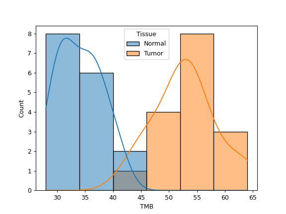
- fuc.api.pyvcf.rescue_filtered_variants(vfs, format='GT')[source]
Rescue filtered variants if they are PASS in at least one of the input VCF files.
- Parameters:
vfs (list) – List of VcfFrame objects.
- Returns:
VcfFrame object.
- Return type:
Examples
>>> from fuc import pyvcf >>> data1 = { ... 'CHROM': ['chr1', 'chr1', 'chr1'], ... 'POS': [100, 101, 102], ... 'ID': ['.', '.', '.'], ... 'REF': ['G', 'T', 'C'], ... 'ALT': ['A', 'C', 'T'], ... 'QUAL': ['.', '.', '.'], ... 'FILTER': ['PASS', 'weak_evidence', 'PASS'], ... 'INFO': ['.', '.', '.'], ... 'FORMAT': ['GT', 'GT', 'GT'], ... 'A': ['0/1', '0/1', '0/1'] ... } >>> data2 = { ... 'CHROM': ['chr1', 'chr1', 'chr1'], ... 'POS': [100, 101, 102], ... 'ID': ['.', '.', '.'], ... 'REF': ['G', 'T', 'C'], ... 'ALT': ['A', 'C', 'T'], ... 'QUAL': ['.', '.', '.'], ... 'FILTER': ['orientation', 'weak_evidence', 'PASS'], ... 'INFO': ['.', '.', '.'], ... 'FORMAT': ['GT', 'GT', 'GT'], ... 'B': ['0/1', '0/1', '0/1'] ... } >>> data3 = { ... 'CHROM': ['chr1', 'chr1', 'chr1'], ... 'POS': [102, 103, 104], ... 'ID': ['.', '.', '.'], ... 'REF': ['C', 'T', 'A'], ... 'ALT': ['T', 'C', 'T'], ... 'QUAL': ['.', '.', '.'], ... 'FILTER': ['PASS', 'weak_evidence', 'PASS'], ... 'INFO': ['.', '.', '.'], ... 'FORMAT': ['GT', 'GT', 'GT'], ... 'C': ['0/1', '0/1', '0/1'] ... } >>> vf1 = pyvcf.VcfFrame.from_dict([], data1) >>> vf2 = pyvcf.VcfFrame.from_dict([], data2) >>> vf3 = pyvcf.VcfFrame.from_dict([], data3) >>> vf1.df CHROM POS ID REF ALT QUAL FILTER INFO FORMAT A 0 chr1 100 . G A . PASS . GT 0/1 1 chr1 101 . T C . weak_evidence . GT 0/1 2 chr1 102 . C T . PASS . GT 0/1 >>> vf2.df CHROM POS ID REF ALT QUAL FILTER INFO FORMAT B 0 chr1 100 . G A . orientation . GT 0/1 1 chr1 101 . T C . weak_evidence . GT 0/1 2 chr1 102 . C T . PASS . GT 0/1 >>> vf3.df CHROM POS ID REF ALT QUAL FILTER INFO FORMAT C 0 chr1 102 . C T . PASS . GT 0/1 1 chr1 103 . T C . weak_evidence . GT 0/1 2 chr1 104 . A T . PASS . GT 0/1 >>> rescued_vf = pyvcf.rescue_filtered_variants([vf1, vf2, vf3]) >>> rescued_vf.df CHROM POS ID REF ALT QUAL FILTER INFO FORMAT A B C 0 chr1 100 . G A . . . GT 0/1 0/1 ./. 1 chr1 102 . C T . . . GT 0/1 0/1 0/1 2 chr1 104 . A T . . . GT ./. ./. 0/1
- fuc.api.pyvcf.row_computeinfo(r, key, decimals=3)[source]
For given row, return AC/AN/AF calculation for INFO column.
- Parameters:
r (pandas.Series) – VCF row.
key ({‘AC’, ‘AN’, ‘AF’}) – INFO key.
decimals (int, default: 3) – Number of decimals to display for AF.
- Returns:
Requested INFO data.
- Return type:
str
Example
>>> from fuc import pyvcf >>> data = { ... 'CHROM': ['chr1', 'chr1', 'chr1', 'chrX'], ... 'POS': [100, 101, 102, 100], ... 'ID': ['.', '.', '.', '.'], ... 'REF': ['G', 'T', 'A', 'A'], ... 'ALT': ['A', 'C', 'T,G', 'G'], ... 'QUAL': ['.', '.', '.', '.'], ... 'FILTER': ['.', '.', '.', '.'], ... 'INFO': ['.', '.', '.', '.'], ... 'FORMAT': ['GT:DP', 'GT', 'GT', 'GT'], ... 'A': ['1|0:29', '0|0', '1|0', '0'], ... 'B': ['1/1:34', './.', '0/0', '0/1'], ... 'C': ['0/0:23', '0/0', '1/2', '1'], ... } >>> vf = pyvcf.VcfFrame.from_dict([], data) >>> vf.df CHROM POS ID REF ALT QUAL FILTER INFO FORMAT A B C 0 chr1 100 . G A . . . GT:DP 1|0:29 1/1:34 0/0:23 1 chr1 101 . T C . . . GT 0|0 ./. 0/0 2 chr1 102 . A T,G . . . GT 1|0 0/0 1/2 3 chrX 100 . A G . . . GT 0 0/1 1 >>> pyvcf.row_computeinfo(vf.df.iloc[0, :], 'AC') '3' >>> pyvcf.row_computeinfo(vf.df.iloc[0, :], 'AN') '6' >>> pyvcf.row_computeinfo(vf.df.iloc[0, :], 'AF') '0.500' >>> pyvcf.row_computeinfo(vf.df.iloc[1, :], 'AC') '0' >>> pyvcf.row_computeinfo(vf.df.iloc[1, :], 'AN') '4' >>> pyvcf.row_computeinfo(vf.df.iloc[1, :], 'AF') '0.000' >>> pyvcf.row_computeinfo(vf.df.iloc[2, :], 'AC') '2,1' >>> pyvcf.row_computeinfo(vf.df.iloc[2, :], 'AN') '6' >>> pyvcf.row_computeinfo(vf.df.iloc[2, :], 'AF') '0.333,0.167' >>> pyvcf.row_computeinfo(vf.df.iloc[3, :], 'AC') '2' >>> pyvcf.row_computeinfo(vf.df.iloc[3, :], 'AN') '4' >>> pyvcf.row_computeinfo(vf.df.iloc[3, :], 'AF') '0.500'
- fuc.api.pyvcf.row_hasindel(r)[source]
For given row, return True if it has indel.
- Parameters:
r (pandas.Series) – VCF row.
- Returns:
True if the row has an indel.
- Return type:
bool
Examples
>>> from fuc import pyvcf >>> data = { ... 'CHROM': ['chr1', 'chr1', 'chr1', 'chr1'], ... 'POS': [100, 101, 102, 103], ... 'ID': ['.', '.', '.', '.'], ... 'REF': ['G', 'CT', 'A', 'C'], ... 'ALT': ['A', 'C', 'C,AT', 'A'], ... 'QUAL': ['.', '.', '.', '.'], ... 'FILTER': ['.', '.', '.', '.'], ... 'INFO': ['.', '.', '.', '.'], ... 'FORMAT': ['GT', 'GT', 'GT', 'GT'], ... 'Steven': ['0/1', '0/1', '1/2', '0/1'], ... } >>> vf = pyvcf.VcfFrame.from_dict([], data) >>> vf.df CHROM POS ID REF ALT QUAL FILTER INFO FORMAT Steven 0 chr1 100 . G A . . . GT 0/1 1 chr1 101 . CT C . . . GT 0/1 2 chr1 102 . A C,AT . . . GT 1/2 3 chr1 103 . C A . . . GT 0/1 >>> vf.df.apply(pyvcf.row_hasindel, axis=1) 0 False 1 True 2 True 3 False dtype: bool
- fuc.api.pyvcf.row_missval(r)[source]
For given row, return formatted missing genotype.
- Parameters:
r (pandas.Series) – VCF row.
- Returns:
Missing value.
- Return type:
str
Examples
>>> from fuc import pyvcf >>> data = { ... 'CHROM': ['chr1', 'chr1', 'chr1', 'chrX'], ... 'POS': [100, 101, 102, 100], ... 'ID': ['.', '.', '.', '.'], ... 'REF': ['G', 'T', 'A', 'C'], ... 'ALT': ['A', 'C', 'T', 'A'], ... 'QUAL': ['.', '.', '.', '.'], ... 'FILTER': ['.', '.', '.', '.'], ... 'INFO': ['.', '.', '.', '.'], ... 'FORMAT': ['GT', 'GT:AD', 'GT:AD:DP', 'GT'], ... 'Steven': ['0/1', '0/1:14,15', '0/1:13,19:32', '0/1'], ... } >>> vf = pyvcf.VcfFrame.from_dict([], data) >>> vf.df CHROM POS ID REF ALT QUAL FILTER INFO FORMAT Steven 0 chr1 100 . G A . . . GT 0/1 1 chr1 101 . T C . . . GT:AD 0/1:14,15 2 chr1 102 . A T . . . GT:AD:DP 0/1:13,19:32 3 chrX 100 . C A . . . GT 0/1 >>> vf.df.apply(pyvcf.row_missval, axis=1) 0 ./. 1 ./.:. 2 ./.:.:. 3 . dtype: object
- fuc.api.pyvcf.row_parseinfo(r, key)[source]
For given row, return requested data from INFO column.
- Parameters:
r (pandas.Series) – VCF row.
key (str) – INFO key.
- Returns:
Requested INFO data. Empty string if the key is not found.
- Return type:
str
Examples
>>> from fuc import pyvcf >>> data = { ... 'CHROM': ['chr1', 'chr1', 'chr1', 'chr1'], ... 'POS': [100, 101, 102, 103], ... 'ID': ['.', '.', '.', '.'], ... 'REF': ['G', 'T', 'A', 'C'], ... 'ALT': ['A', 'C', 'T', 'A'], ... 'QUAL': ['.', '.', '.', '.'], ... 'FILTER': ['.', '.', '.', '.'], ... 'INFO': ['DB;AC=0', 'DB;H2;AC=1', 'DB;H2;AC=1', '.'], ... 'FORMAT': ['GT', 'GT', 'GT', 'GT'], ... 'Steven': ['0/0', '0/1', '0/1', '0/0'], ... } >>> vf = pyvcf.VcfFrame.from_dict([], data) >>> vf.df CHROM POS ID REF ALT QUAL FILTER INFO FORMAT Steven 0 chr1 100 . G A . . DB;AC=0 GT 0/0 1 chr1 101 . T C . . DB;H2;AC=1 GT 0/1 2 chr1 102 . A T . . DB;H2;AC=1 GT 0/1 3 chr1 103 . C A . . . GT 0/0 >>> vf.df.apply(pyvcf.row_parseinfo, args=('AC',), axis=1) 0 0 1 1 2 1 3 dtype: object
- fuc.api.pyvcf.row_phased(r)[source]
For given row, return True if all genotypes are phased.
- Parameters:
r (pandas.Series) – VCF row.
- Returns:
True if the row is fully phased.
- Return type:
bool
Examples
>>> data = { ... 'CHROM': ['chr1', 'chr1', 'chr1'], ... 'POS': [100, 101, 102], ... 'ID': ['.', '.', '.'], ... 'REF': ['G', 'T', 'A'], ... 'ALT': ['A', 'C', 'T'], ... 'QUAL': ['.', '.', '.'], ... 'FILTER': ['.', '.', '.'], ... 'INFO': ['.', '.', '.'], ... 'FORMAT': ['GT', 'GT', 'GT'], ... 'A': ['1|1', '0/0', '1|0'], ... 'B': ['1|0', '0/1', '1/0'], ... } >>> vf = pyvcf.VcfFrame.from_dict([], data) >>> vf.df CHROM POS ID REF ALT QUAL FILTER INFO FORMAT A B 0 chr1 100 . G A . . . GT 1|1 1|0 1 chr1 101 . T C . . . GT 0/0 0/1 2 chr1 102 . A T . . . GT 1|0 1/0 >>> vf.df.apply(pyvcf.row_phased, axis=1) 0 True 1 False 2 False dtype: bool
- fuc.api.pyvcf.row_updateinfo(r, key, value, force=True, missing=False)[source]
For given row, return updated data from INFO column.
- Parameters:
r (pandas.Series) – VCF row.
key (str) – INFO key.
value (str) – New value to be assigned.
force (bool, default: True) – If True, overwrite any existing data.
missing (bool, default: False) – By default (
missing=False), the method will not update INFO field if there is missing value (‘.’). Settingmissing=Truewill stop this behavior.
- Returns:
New INFO field.
- Return type:
str
Examples
>>> from fuc import pyvcf >>> data = { ... 'CHROM': ['chr1', 'chr1', 'chr1'], ... 'POS': [100, 101, 102], ... 'ID': ['.', '.', '.'], ... 'REF': ['G', 'T', 'A'], ... 'ALT': ['A', 'C', 'T'], ... 'QUAL': ['.', '.', '.'], ... 'FILTER': ['.', '.', '.'], ... 'INFO': ['DB;AC=1', 'DB', '.'], ... 'FORMAT': ['GT', 'GT', 'GT'], ... 'A': ['0/1', '1/1', '0/0'], ... 'B': ['0/0', '0/1', '0/1'], ... } >>> vf = pyvcf.VcfFrame.from_dict([], data) >>> vf.df CHROM POS ID REF ALT QUAL FILTER INFO FORMAT A B 0 chr1 100 . G A . . DB;AC=1 GT 0/1 0/0 1 chr1 101 . T C . . DB GT 1/1 0/1 2 chr1 102 . A T . . . GT 0/0 0/1 >>> pyvcf.row_updateinfo(vf.df.iloc[0, :], 'AC', '100') 'DB;AC=100' >>> pyvcf.row_updateinfo(vf.df.iloc[0, :], 'AC', '100', force=False) 'DB;AC=1' >>> pyvcf.row_updateinfo(vf.df.iloc[1, :], 'AC', '100') 'DB;AC=100' >>> pyvcf.row_updateinfo(vf.df.iloc[1, :], 'AC', '100', force=False) 'DB;AC=100' >>> pyvcf.row_updateinfo(vf.df.iloc[2, :], 'AC', '100') '.' >>> pyvcf.row_updateinfo(vf.df.iloc[2, :], 'AC', '100', force=False) '.' >>> pyvcf.row_updateinfo(vf.df.iloc[2, :], 'AC', '100', missing=True) 'AC=100'
- fuc.api.pyvcf.slice(file, regions, path=None)[source]
Slice a VCF file for specified regions.
- Parameters:
file (str) – Input VCF file must be already BGZF compressed (.gz) and indexed (.tbi) to allow random access.
regions (str, list, or pybed.BedFrame) – One or more regions to be sliced. Each region must have the format chrom:start-end and be a half-open interval with (start, end]. This means, for example, chr1:100-103 will extract positions 101, 102, and 103. Alternatively, you can provide a BED file (compressed or uncompressed) to specify regions. Note that the ‘chr’ prefix in contig names (e.g. ‘chr1’ vs. ‘1’) will be automatically added or removed as necessary to match the input VCF’s contig names.
path (str, optional) – Output VCF file. Writes to stdout when
path='-'. If None is provided the result is returned as a string.
- Returns:
If
pathis None, returns the resulting VCF format as a string. Otherwise returns None.- Return type:
None or str
- fuc.api.pyvcf.split(vcf, clean=True)[source]
Split VcfFrame by individual.
- Parameters:
vcf (str or VcfFrame) – VCF file or VcfFrame to be split.
clean (bool, default: True) – If True, only return variants present in each individual. In other words, setting this as False will make sure that all individuals have the same number of variants.
- Returns:
List of individual VcfFrames.
- Return type:
list
Examples
>>> from fuc import pyvcf >>> data = { ... 'CHROM': ['chr1', 'chr1'], ... 'POS': [100, 101], ... 'ID': ['.', '.'], ... 'REF': ['G', 'T'], ... 'ALT': ['A', 'C'], ... 'QUAL': ['.', '.'], ... 'FILTER': ['.', '.'], ... 'INFO': ['.', '.'], ... 'FORMAT': ['GT', 'GT'], ... 'A': ['0/1', '0/0'], ... 'B': ['0/1', '0/1'], ... } >>> vf = pyvcf.VcfFrame.from_dict(['##fileformat=VCFv4.3'], data) >>> vf.df CHROM POS ID REF ALT QUAL FILTER INFO FORMAT A B 0 chr1 100 . G A . . . GT 0/1 0/1 1 chr1 101 . T C . . . GT 0/0 0/1 >>> vfs = pyvcf.split(vf) >>> vfs[0].df CHROM POS ID REF ALT QUAL FILTER INFO FORMAT A 0 chr1 100 . G A . . . GT 0/1 >>> vfs = pyvcf.split(vf, clean=False) >>> vfs[0].df CHROM POS ID REF ALT QUAL FILTER INFO FORMAT A 0 chr1 100 . G A . . . GT 0/1 1 chr1 101 . T C . . . GT 0/0
fuc.pyvep
The pyvep submodule is designed for parsing VCF annotation data from the
Ensembl VEP
program. It should be used with pyvcf.VcfFrame.
The input VCF should already contain functional annotation data from Ensembl VEP. The recommended method is Ensembl VEP’s web interface with “RefSeq transcripts” as the transcript database and the filtering option “Show one selected consequence per variant”.
A typical VEP-annotated VCF file contains many fields ranging from gene symbol to protein change. However, most of the analysis in pyvep uses the following fields:
No. |
Name |
Description |
Examples |
|---|---|---|---|
1 |
Allele |
Variant allele |
‘C’, ‘T’, ‘CG’ |
2 |
Consequence |
Consequence type |
‘missense_variant’, ‘stop_gained’ |
3 |
IMPACT |
Consequence impact |
‘MODERATE’, ‘HIGH’ |
4 |
SYMBOL |
Gene symbol |
‘TP53’, ‘APC’ |
5 |
Gene |
Ensembl ID |
7157, 55294 |
6 |
BIOTYPE |
Transcript biotype |
‘protein_coding’, ‘pseudogene’, ‘miRNA’ |
7 |
EXON |
Exon number |
‘8/17’, ‘17/17’ |
8 |
Protein_position |
Amino acid position |
234, 1510 |
9 |
Amino_acids |
Amino acid changes |
‘R/*’, ‘A/X’, ‘V/A’ |
10 |
Existing_variation |
Variant identifier |
‘rs17851045’, ‘rs786201856&COSV57325157’ |
11 |
STRAND |
Genomic strand |
1, -1 |
12 |
SIFT |
SIFT prediction |
‘tolerated(0.6)’, ‘tolerated_low_confidence(0.37)’, ‘deleterious_low_confidence(0.03)’, ‘deleterious(0)’ |
13 |
PolyPhen |
PolyPhen prediction |
‘benign(0.121)’, ‘possibly_damaging(0.459)’, ‘probably_damaging(0.999)’ |
14 |
CLIN_SIG |
ClinVar prediction |
‘pathogenic’, ‘likely_pathogenic&pathogenic’ |
Functions:
|
Return the list of avaialble consequence annotations in the VcfFrame. |
|
Select rows that satisfy the query expression. |
|
Parse variant annotations in VcfFrame. |
|
Return a new VcfFrame after picking one result per row. |
|
Return the first result in the row. |
Return result with the most severe consequence in the row. |
|
|
Create a DataFrame containing analysis-ready VEP annotation data. |
- fuc.api.pyvep.annot_names(vf)[source]
Return the list of avaialble consequence annotations in the VcfFrame.
- Parameters:
vf (VcfFrame) – VcfFrame.
- Returns:
List of consequence annotations.
- Return type:
list
- fuc.api.pyvep.filter_query(vf, expr, opposite=None, as_index=False, as_zero=False)[source]
Select rows that satisfy the query expression.
This method essentially wraps the
pandas.DataFrame.query()method.- Parameters:
expr (str) – The query string to evaluate.
opposite (bool, default: False) – If True, return rows that don’t meet the said criteria.
as_index (bool, default: False) – If True, return boolean index array instead of VcfFrame.
as_zero (bool, default: False) – If True, missing values will be converted to zeros instead of
NaN.
- Returns:
Filtered VcfFrame or boolean index array.
- Return type:
VcfFrame or pandas.Series
Examples
>>> from fuc import common, pyvcf, pyvep >>> common.load_dataset('tcga-laml') >>> fn = '~/fuc-data/tcga-laml/tcga_laml_vep.vcf' >>> vf = pyvcf.VcfFrame.from_file(fn) >>> filtered_vf = pyvep.filter_query(vf, "SYMBOL == 'TP53'") >>> filtered_vf = pyvep.filter_query(vf, "SYMBOL != 'TP53'") >>> filtered_vf = pyvep.filter_query(vf, "SYMBOL != 'TP53'", opposite=True) >>> filtered_vf = pyvep.filter_query(vf, "Consequence in ['splice_donor_variant', 'stop_gained']") >>> filtered_vf = pyvep.filter_query(vf, "(SYMBOL == 'TP53') and (Consequence.str.contains('stop_gained'))") >>> filtered_vf = pyvep.filter_query(vf, "gnomAD_AF < 0.001") >>> filtered_vf = pyvep.filter_query(vf, "gnomAD_AF < 0.001", as_zero=True) >>> filtered_vf = pyvep.filter_query(vf, "(IMPACT == 'HIGH') or (Consequence.str.contains('missense_variant') and (PolyPhen.str.contains('damaging') or SIFT.str.contains('deleterious')))")
- fuc.api.pyvep.parseann(vf, targets, sep=' | ', as_series=False)[source]
Parse variant annotations in VcfFrame.
If there are multiple results per row, the method will use the first one for extracting requested data.
- Parameters:
vf (VcfFrame) – VcfFrame.
targets (list) – List of subfield IDs or indicies or both.
sep (str, default: ‘ | ‘) – Separator for joining requested annotations.
as_series (bool, default: False) – If True, return 1D array instead of VcfFrame.
- Returns:
Parsed annotations in VcfFrame or 1D array.
- Return type:
VcfFrame or pandas.Series
Examples
Assume we have the following data:
>>> meta = [ ... '##fileformat=VCFv4.1', ... '##VEP="v104" time="2021-05-20 10:50:12" cache="/net/isilonP/public/ro/ensweb-data/latest/tools/grch37/e104/vep/cache/homo_sapiens/104_GRCh37" db="homo_sapiens_core_104_37@hh-mysql-ens-grch37-web" 1000genomes="phase3" COSMIC="92" ClinVar="202012" HGMD-PUBLIC="20204" assembly="GRCh37.p13" dbSNP="154" gencode="GENCODE 19" genebuild="2011-04" gnomAD="r2.1" polyphen="2.2.2" regbuild="1.0" sift="sift5.2.2"', ... '##INFO=<ID=CSQ,Number=.,Type=String,Description="Consequence annotations from Ensembl VEP. Format: Allele|Consequence|IMPACT|SYMBOL|Gene|Feature_type|Feature|BIOTYPE|EXON|INTRON|HGVSc|HGVSp|cDNA_position|CDS_position|Protein_position|Amino_acids|Codons|Existing_variation|DISTANCE|STRAND|FLAGS|SYMBOL_SOURCE|HGNC_ID|MANE_SELECT|MANE_PLUS_CLINICAL|TSL|APPRIS|SIFT|PolyPhen|AF|CLIN_SIG|SOMATIC|PHENO|PUBMED|MOTIF_NAME|MOTIF_POS|HIGH_INF_POS|MOTIF_SCORE_CHANGE|TRANSCRIPTION_FACTORS">' ... ] >>> data = { ... 'CHROM': ['chr1', 'chr1', 'chr2', 'chr2'], ... 'POS': [100, 101, 200, 201], ... 'ID': ['.', '.', '.', '.'], ... 'REF': ['G', 'C', 'CAG', 'C'], ... 'ALT': ['T', 'T', 'C', 'T'], ... 'QUAL': ['.', '.', '.', '.'], ... 'FILTER': ['.', '.', '.', '.'], ... 'INFO': [ ... 'CSQ=T|missense_variant|MODERATE|MTOR|ENSG00000198793|Transcript|ENST00000361445.4|protein_coding|47/58||||6721|6644|2215|S/Y|tCt/tAt|rs587777894&COSV63868278&COSV63868313||-1||HGNC|3942|||||deleterious(0)|possibly_damaging(0.876)||likely_pathogenic&pathogenic|0&1&1|1&1&1|26619011&27159400&24631838&26018084&27830187|||||', ... 'CSQ=T|synonymous_variant|LOW|MTOR|ENSG00000198793|Transcript|ENST00000361445.4|protein_coding|49/58||||6986|6909|2303|L|ctG/ctA|rs11121691&COSV63870864||-1||HGNC|3942|||||||0.2206|benign|0&1|1&1|24996771|||||', ... 'CSQ=-|frameshift_variant|HIGH|BRCA2|ENSG00000139618|Transcript|ENST00000380152.3|protein_coding|18/27||||8479-8480|8246-8247|2749|Q/X|cAG/c|rs80359701||1||HGNC|1101||||||||pathogenic||1|26467025&26295337&15340362|||||', ... 'CSQ=T|missense_variant|MODERATE|MTOR|ENSG00000198793|Transcript|ENST00000361445.4|protein_coding|30/58||||4516|4439|1480|R/H|cGc/cAc|rs780930764&COSV63868373||-1||HGNC|3942|||||tolerated(0.13)|benign(0)||likely_benign|0&1|1&1||||||' ... ], ... 'FORMAT': ['GT', 'GT', 'GT', 'GT'], ... 'Steven': ['0/1', '0/1', '0/1', '0/1'], ... } >>> vf = pyvcf.VcfFrame.from_dict(meta, data)
We can extract gene symbols:
>>> pyvep.parseann(vf, ['SYMBOL']).df CHROM POS ID REF ALT QUAL FILTER INFO FORMAT Steven 0 chr1 100 . G T . . MTOR GT 0/1 1 chr1 101 . C T . . MTOR GT 0/1 2 chr2 200 . CAG C . . BRCA2 GT 0/1 3 chr2 201 . C T . . MTOR GT 0/1
If we want to add variant impact:
>>> pyvep.parseann(vf, ['SYMBOL', 'IMPACT']).df CHROM POS ID REF ALT QUAL FILTER INFO FORMAT Steven 0 chr1 100 . G T . . MTOR | MODERATE GT 0/1 1 chr1 101 . C T . . MTOR | LOW GT 0/1 2 chr2 200 . CAG C . . BRCA2 | HIGH GT 0/1 3 chr2 201 . C T . . MTOR | MODERATE GT 0/1
If we want to change the delimter:
>>> pyvep.parseann(vf, ['SYMBOL', 'IMPACT'], sep=',').df CHROM POS ID REF ALT QUAL FILTER INFO FORMAT Steven 0 chr1 100 . G T . . MTOR,MODERATE GT 0/1 1 chr1 101 . C T . . MTOR,LOW GT 0/1 2 chr2 200 . CAG C . . BRCA2,HIGH GT 0/1 3 chr2 201 . C T . . MTOR,MODERATE GT 0/1
Finally, we can return a 1D array instead of VcfFrame:
>>> pyvep.parseann(vf, ['SYMBOL'], as_series=True) 0 MTOR 1 MTOR 2 BRCA2 3 MTOR dtype: object
- fuc.api.pyvep.pick_result(vf, mode='mostsevere')[source]
Return a new VcfFrame after picking one result per row.
- Parameters:
vf (VcfFrame) – VcfFrame object.
mode ({‘mostsevere’, ‘firstann’}, default: ‘mostsevere’) –
Selection mode:
mostsevere: use
row_mostseveremethodfirstann: use
row_firstannmethod
- Returns:
New VcfFrame.
- Return type:
Examples
>>> from fuc import pyvep, pyvcf >>> meta = [ ... '##fileformat=VCFv4.1', ... '##VEP="v104" time="2021-05-20 10:50:12" cache="/net/isilonP/public/ro/ensweb-data/latest/tools/grch37/e104/vep/cache/homo_sapiens/104_GRCh37" db="homo_sapiens_core_104_37@hh-mysql-ens-grch37-web" 1000genomes="phase3" COSMIC="92" ClinVar="202012" HGMD-PUBLIC="20204" assembly="GRCh37.p13" dbSNP="154" gencode="GENCODE 19" genebuild="2011-04" gnomAD="r2.1" polyphen="2.2.2" regbuild="1.0" sift="sift5.2.2"', ... '##INFO=<ID=CSQ,Number=.,Type=String,Description="Consequence annotations from Ensembl VEP. Format: Allele|Consequence|IMPACT|SYMBOL|Gene|Feature_type|Feature|BIOTYPE|EXON|INTRON|HGVSc|HGVSp|cDNA_position|CDS_position|Protein_position|Amino_acids|Codons|Existing_variation|DISTANCE|STRAND|FLAGS|SYMBOL_SOURCE|HGNC_ID|MANE_SELECT|MANE_PLUS_CLINICAL|TSL|APPRIS|SIFT|PolyPhen|AF|CLIN_SIG|SOMATIC|PHENO|PUBMED|MOTIF_NAME|MOTIF_POS|HIGH_INF_POS|MOTIF_SCORE_CHANGE|TRANSCRIPTION_FACTORS">' ... ] >>> data = { ... 'CHROM': ['chr1', 'chr1', 'chr2', 'chr2'], ... 'POS': [100, 101, 200, 201], ... 'ID': ['.', '.', '.', '.'], ... 'REF': ['G', 'C', 'G', 'CCCA'], ... 'ALT': ['C', 'T', 'A', 'C'], ... 'QUAL': ['.', '.', '.', '.'], ... 'FILTER': ['.', '.', '.', '.'], ... 'INFO': [ ... 'CSQ=C|downstream_gene_variant|MODIFIER|ZBTB17|ENSG00000116809|Transcript|ENST00000375733.2|protein_coding|||||||||||4617|-1||HGNC|12936||||||||||||||||,C|downstream_gene_variant|MODIFIER|ZBTB17|ENSG00000116809|Transcript|ENST00000375743.4|protein_coding|||||||||||4615|-1||HGNC|12936||||||||||||||||,C|missense_variant|MODERATE|SPEN|ENSG00000065526|Transcript|ENST00000375759.3|protein_coding|12/15||||10322|10118|3373|Q/P|cAg/cCg|||1||HGNC|17575|||||tolerated_low_confidence(0.08)|possibly_damaging(0.718)||||||||||,C|downstream_gene_variant|MODIFIER|ZBTB17|ENSG00000116809|Transcript|ENST00000440560.1|protein_coding|||||||||||4615|-1|cds_start_NF|HGNC|12936||||||||||||||||,C|downstream_gene_variant|MODIFIER|ZBTB17|ENSG00000116809|Transcript|ENST00000462525.1|processed_transcript|||||||||||4615|-1||HGNC|12936||||||||||||||||,C|upstream_gene_variant|MODIFIER|SPEN|ENSG00000065526|Transcript|ENST00000487496.1|processed_transcript|||||||||||1329|1||HGNC|17575||||||||||||||||,C|downstream_gene_variant|MODIFIER|ZBTB17|ENSG00000116809|Transcript|ENST00000537142.1|protein_coding|||||||||||4617|-1||HGNC|12936||||||||||||||||,C|regulatory_region_variant|MODIFIER|||RegulatoryFeature|ENSR00000922256|promoter_flanking_region|||||||||||||||||||||||||||||||', ... 'CSQ=T|downstream_gene_variant|MODIFIER|CSDE1|ENSG00000009307|Transcript|ENST00000261443.5|protein_coding||||||||||COSV99795232|3453|-1||HGNC|29905|||||||||1|1||||||,T|downstream_gene_variant|MODIFIER|CSDE1|ENSG00000009307|Transcript|ENST00000339438.6|protein_coding||||||||||COSV99795232|3071|-1||HGNC|29905|||||||||1|1||||||,T|downstream_gene_variant|MODIFIER|CSDE1|ENSG00000009307|Transcript|ENST00000358528.4|protein_coding||||||||||COSV99795232|3075|-1||HGNC|29905|||||||||1|1||||||,T|downstream_gene_variant|MODIFIER|CSDE1|ENSG00000009307|Transcript|ENST00000369530.1|protein_coding||||||||||COSV99795232|3470|-1||HGNC|29905|||||||||1|1||||||,T|missense_variant|MODERATE|NRAS|ENSG00000213281|Transcript|ENST00000369535.4|protein_coding|3/7||||502|248|83|A/D|gCc/gAc|COSV99795232||-1||HGNC|7989|||||deleterious(0.02)|probably_damaging(0.946)|||1|1||||||,T|downstream_gene_variant|MODIFIER|CSDE1|ENSG00000009307|Transcript|ENST00000438362.2|protein_coding||||||||||COSV99795232|3074|-1||HGNC|29905|||||||||1|1||||||,T|downstream_gene_variant|MODIFIER|CSDE1|ENSG00000009307|Transcript|ENST00000483407.1|processed_transcript||||||||||COSV99795232|3960|-1||HGNC|29905|||||||||1|1||||||,T|downstream_gene_variant|MODIFIER|CSDE1|ENSG00000009307|Transcript|ENST00000530886.1|protein_coding||||||||||COSV99795232|3463|-1||HGNC|29905|||||||||1|1||||||,T|downstream_gene_variant|MODIFIER|CSDE1|ENSG00000009307|Transcript|ENST00000534699.1|protein_coding||||||||||COSV99795232|4115|-1||HGNC|29905|||||||||1|1||||||', ... 'CSQ=A|missense_variant|MODERATE|NTRK1|ENSG00000198400|Transcript|ENST00000358660.3|protein_coding|10/16||||1296|1255|419|A/T|Gcc/Acc|COSV62328771||1||HGNC|8031|||||deleterious(0.01)|probably_damaging(0.999)|||1|1||||||,A|missense_variant|MODERATE|NTRK1|ENSG00000198400|Transcript|ENST00000368196.3|protein_coding|10/16||||1375|1255|419|A/T|Gcc/Acc|COSV62328771||1||HGNC|8031|||||deleterious(0.01)|possibly_damaging(0.894)|||1|1||||||,A|missense_variant|MODERATE|NTRK1|ENSG00000198400|Transcript|ENST00000392302.2|protein_coding|11/17||||1339|1165|389|A/T|Gcc/Acc|COSV62328771||1||HGNC|8031|||||deleterious(0.01)|probably_damaging(0.983)|||1|1||||||,A|downstream_gene_variant|MODIFIER|NTRK1|ENSG00000198400|Transcript|ENST00000489021.2|processed_transcript||||||||||COSV62328771|1037|1||HGNC|8031|||||||||1|1||||||,A|stop_gained&NMD_transcript_variant|HIGH|NTRK1|ENSG00000198400|Transcript|ENST00000497019.2|nonsense_mediated_decay|10/16||||1183|1032|344|W/*|tgG/tgA|COSV62328771||1||HGNC|8031|||||||||1|1||||||,A|missense_variant|MODERATE|NTRK1|ENSG00000198400|Transcript|ENST00000524377.1|protein_coding|11/17||||1314|1273|425|A/T|Gcc/Acc|COSV62328771||1||HGNC|8031|||||deleterious(0.01)|probably_damaging(0.996)|||1|1||||||,A|non_coding_transcript_exon_variant|MODIFIER|NTRK1|ENSG00000198400|Transcript|ENST00000530298.1|retained_intron|12/17||||1313|||||COSV62328771||1||HGNC|8031|||||||||1|1||||||,A|non_coding_transcript_exon_variant|MODIFIER|NTRK1|ENSG00000198400|Transcript|ENST00000534682.1|retained_intron|2/4||||496|||||COSV62328771||1||HGNC|8031|||||||||1|1||||||,A|regulatory_region_variant|MODIFIER|||RegulatoryFeature|ENSR00001787924|open_chromatin_region||||||||||COSV62328771||||||||||||||1|1||||||', ... 'CSQ=-|upstream_gene_variant|MODIFIER|LRRC56|ENSG00000161328|Transcript|ENST00000270115.7|protein_coding||||||||||rs1164486792|3230|1||HGNC|25430||||||||||1||||||,-|inframe_deletion|MODERATE|HRAS|ENSG00000174775|Transcript|ENST00000311189.7|protein_coding|2/6||||198-200|26-28|9-10|VG/G|gTGGgc/ggc|rs1164486792||-1||HGNC|5173||||||||||1||||||,-|inframe_deletion|MODERATE|HRAS|ENSG00000174775|Transcript|ENST00000397594.1|protein_coding|1/5||||79-81|26-28|9-10|VG/G|gTGGgc/ggc|rs1164486792||-1||HGNC|5173||||||||||1||||||,-|inframe_deletion|MODERATE|HRAS|ENSG00000174775|Transcript|ENST00000397596.2|protein_coding|2/5||||162-164|26-28|9-10|VG/G|gTGGgc/ggc|rs1164486792||-1||HGNC|5173||||||||||1||||||,-|inframe_deletion|MODERATE|HRAS|ENSG00000174775|Transcript|ENST00000417302.1|protein_coding|2/6||||214-216|26-28|9-10|VG/G|gTGGgc/ggc|rs1164486792||-1||HGNC|5173||||||||||1||||||,-|inframe_deletion|MODERATE|HRAS|ENSG00000174775|Transcript|ENST00000451590.1|protein_coding|2/5||||214-216|26-28|9-10|VG/G|gTGGgc/ggc|rs1164486792||-1||HGNC|5173||||||||||1||||||,-|upstream_gene_variant|MODIFIER|HRAS|ENSG00000174775|Transcript|ENST00000462734.1|processed_transcript||||||||||rs1164486792|700|-1||HGNC|5173||||||||||1||||||,-|non_coding_transcript_exon_variant|MODIFIER|HRAS|ENSG00000174775|Transcript|ENST00000468682.2|processed_transcript|2/3||||514-516|||||rs1164486792||-1||HGNC|5173||||||||||1||||||,-|upstream_gene_variant|MODIFIER|HRAS|ENSG00000174775|Transcript|ENST00000478324.1|processed_transcript||||||||||rs1164486792|683|-1||HGNC|5173||||||||||1||||||,-|upstream_gene_variant|MODIFIER|HRAS|ENSG00000174775|Transcript|ENST00000479482.1|processed_transcript||||||||||rs1164486792|319|-1||HGNC|5173||||||||||1||||||,-|non_coding_transcript_exon_variant|MODIFIER|HRAS|ENSG00000174775|Transcript|ENST00000482021.1|processed_transcript|2/2||||149-151|||||rs1164486792||-1||HGNC|5173||||||||||1||||||,-|inframe_deletion&NMD_transcript_variant|MODERATE|HRAS|ENSG00000174775|Transcript|ENST00000493230.1|nonsense_mediated_decay|2/7||||202-204|26-28|9-10|VG/G|gTGGgc/ggc|rs1164486792||-1||HGNC|5173||||||||||1||||||,-|downstream_gene_variant|MODIFIER|RP13-46H24.1|ENSG00000254739|Transcript|ENST00000526431.1|antisense||||||||||rs1164486792|4636|1||Clone_based_vega_gene|||||||||||1||||||,-|regulatory_region_variant|MODIFIER|||RegulatoryFeature|ENSR00000035647|promoter||||||||||rs1164486792|||||||||||||||1||||||' ... ], ... 'FORMAT': ['GT', 'GT', 'GT', 'GT'], ... 'Steven': ['0/1', '0/1', '0/1', '0/1'], ... } >>> vf = pyvcf.VcfFrame.from_dict(meta, data) >>> vf1 = pyvep.pick_result(vf, mode='mostsevere') >>> vf2 = pyvep.pick_result(vf, mode='firstann') >>> vf1.df.INFO 0 CSQ=C|missense_variant|MODERATE|SPEN|ENSG00000065526|Transcript|ENST00000375759.3|protein_coding|12/15||||10322|10118|3373|Q/P|cAg/cCg|||1||HGNC|17575|||||tolerated_low_confidence(0.08)|possibly_damaging(0.718)|||||||||| 1 CSQ=T|missense_variant|MODERATE|NRAS|ENSG00000213281|Transcript|ENST00000369535.4|protein_coding|3/7||||502|248|83|A/D|gCc/gAc|COSV99795232||-1||HGNC|7989|||||deleterious(0.02)|probably_damaging(0.946)|||1|1|||||| 2 CSQ=A|stop_gained&NMD_transcript_variant|HIGH|NTRK1|ENSG00000198400|Transcript|ENST00000497019.2|nonsense_mediated_decay|10/16||||1183|1032|344|W/*|tgG/tgA|COSV62328771||1||HGNC|8031|||||||||1|1|||||| 3 CSQ=-|inframe_deletion|MODERATE|HRAS|ENSG00000174775|Transcript|ENST00000311189.7|protein_coding|2/6||||198-200|26-28|9-10|VG/G|gTGGgc/ggc|rs1164486792||-1||HGNC|5173||||||||||1|||||| Name: INFO, dtype: object >>> vf2.df.INFO 0 CSQ=C|downstream_gene_variant|MODIFIER|ZBTB17|ENSG00000116809|Transcript|ENST00000375733.2|protein_coding|||||||||||4617|-1||HGNC|12936|||||||||||||||| 1 CSQ=T|downstream_gene_variant|MODIFIER|CSDE1|ENSG00000009307|Transcript|ENST00000261443.5|protein_coding||||||||||COSV99795232|3453|-1||HGNC|29905|||||||||1|1|||||| 2 CSQ=A|missense_variant|MODERATE|NTRK1|ENSG00000198400|Transcript|ENST00000358660.3|protein_coding|10/16||||1296|1255|419|A/T|Gcc/Acc|COSV62328771||1||HGNC|8031|||||deleterious(0.01)|probably_damaging(0.999)|||1|1|||||| 3 CSQ=-|upstream_gene_variant|MODIFIER|LRRC56|ENSG00000161328|Transcript|ENST00000270115.7|protein_coding||||||||||rs1164486792|3230|1||HGNC|25430||||||||||1|||||| Name: INFO, dtype: object
- fuc.api.pyvep.row_firstann(r)[source]
Return the first result in the row.
- Parameters:
r (pandas.Series) – VCF row.
- Returns:
Annotation result. Empty string if annotation is not found.
- Return type:
str
See also
row_mostsevereSimilar method that returns result with the most severe consequence in the row.
Examples
>>> data = { ... 'CHROM': ['chr1', 'chr1', 'chr2', 'chr2'], ... 'POS': [100, 101, 200, 201], ... 'ID': ['.', '.', '.', '.'], ... 'REF': ['G', 'C', 'G', 'CCCA'], ... 'ALT': ['C', 'T', 'A', 'C'], ... 'QUAL': ['.', '.', '.', '.'], ... 'FILTER': ['.', '.', '.', '.'], ... 'INFO': [ ... 'CSQ=C|downstream_gene_variant|MODIFIER|ZBTB17|ENSG00000116809|Transcript|ENST00000375733.2|protein_coding|||||||||||4617|-1||HGNC|12936||||||||||||||||,C|downstream_gene_variant|MODIFIER|ZBTB17|ENSG00000116809|Transcript|ENST00000375743.4|protein_coding|||||||||||4615|-1||HGNC|12936||||||||||||||||,C|missense_variant|MODERATE|SPEN|ENSG00000065526|Transcript|ENST00000375759.3|protein_coding|12/15||||10322|10118|3373|Q/P|cAg/cCg|||1||HGNC|17575|||||tolerated_low_confidence(0.08)|possibly_damaging(0.718)||||||||||,C|downstream_gene_variant|MODIFIER|ZBTB17|ENSG00000116809|Transcript|ENST00000440560.1|protein_coding|||||||||||4615|-1|cds_start_NF|HGNC|12936||||||||||||||||,C|downstream_gene_variant|MODIFIER|ZBTB17|ENSG00000116809|Transcript|ENST00000462525.1|processed_transcript|||||||||||4615|-1||HGNC|12936||||||||||||||||,C|upstream_gene_variant|MODIFIER|SPEN|ENSG00000065526|Transcript|ENST00000487496.1|processed_transcript|||||||||||1329|1||HGNC|17575||||||||||||||||,C|downstream_gene_variant|MODIFIER|ZBTB17|ENSG00000116809|Transcript|ENST00000537142.1|protein_coding|||||||||||4617|-1||HGNC|12936||||||||||||||||,C|regulatory_region_variant|MODIFIER|||RegulatoryFeature|ENSR00000922256|promoter_flanking_region|||||||||||||||||||||||||||||||', ... 'CSQ=T|downstream_gene_variant|MODIFIER|CSDE1|ENSG00000009307|Transcript|ENST00000261443.5|protein_coding||||||||||COSV99795232|3453|-1||HGNC|29905|||||||||1|1||||||,T|downstream_gene_variant|MODIFIER|CSDE1|ENSG00000009307|Transcript|ENST00000339438.6|protein_coding||||||||||COSV99795232|3071|-1||HGNC|29905|||||||||1|1||||||,T|downstream_gene_variant|MODIFIER|CSDE1|ENSG00000009307|Transcript|ENST00000358528.4|protein_coding||||||||||COSV99795232|3075|-1||HGNC|29905|||||||||1|1||||||,T|downstream_gene_variant|MODIFIER|CSDE1|ENSG00000009307|Transcript|ENST00000369530.1|protein_coding||||||||||COSV99795232|3470|-1||HGNC|29905|||||||||1|1||||||,T|missense_variant|MODERATE|NRAS|ENSG00000213281|Transcript|ENST00000369535.4|protein_coding|3/7||||502|248|83|A/D|gCc/gAc|COSV99795232||-1||HGNC|7989|||||deleterious(0.02)|probably_damaging(0.946)|||1|1||||||,T|downstream_gene_variant|MODIFIER|CSDE1|ENSG00000009307|Transcript|ENST00000438362.2|protein_coding||||||||||COSV99795232|3074|-1||HGNC|29905|||||||||1|1||||||,T|downstream_gene_variant|MODIFIER|CSDE1|ENSG00000009307|Transcript|ENST00000483407.1|processed_transcript||||||||||COSV99795232|3960|-1||HGNC|29905|||||||||1|1||||||,T|downstream_gene_variant|MODIFIER|CSDE1|ENSG00000009307|Transcript|ENST00000530886.1|protein_coding||||||||||COSV99795232|3463|-1||HGNC|29905|||||||||1|1||||||,T|downstream_gene_variant|MODIFIER|CSDE1|ENSG00000009307|Transcript|ENST00000534699.1|protein_coding||||||||||COSV99795232|4115|-1||HGNC|29905|||||||||1|1||||||', ... 'CSQ=A|missense_variant|MODERATE|NTRK1|ENSG00000198400|Transcript|ENST00000358660.3|protein_coding|10/16||||1296|1255|419|A/T|Gcc/Acc|COSV62328771||1||HGNC|8031|||||deleterious(0.01)|probably_damaging(0.999)|||1|1||||||,A|missense_variant|MODERATE|NTRK1|ENSG00000198400|Transcript|ENST00000368196.3|protein_coding|10/16||||1375|1255|419|A/T|Gcc/Acc|COSV62328771||1||HGNC|8031|||||deleterious(0.01)|possibly_damaging(0.894)|||1|1||||||,A|missense_variant|MODERATE|NTRK1|ENSG00000198400|Transcript|ENST00000392302.2|protein_coding|11/17||||1339|1165|389|A/T|Gcc/Acc|COSV62328771||1||HGNC|8031|||||deleterious(0.01)|probably_damaging(0.983)|||1|1||||||,A|downstream_gene_variant|MODIFIER|NTRK1|ENSG00000198400|Transcript|ENST00000489021.2|processed_transcript||||||||||COSV62328771|1037|1||HGNC|8031|||||||||1|1||||||,A|stop_gained&NMD_transcript_variant|HIGH|NTRK1|ENSG00000198400|Transcript|ENST00000497019.2|nonsense_mediated_decay|10/16||||1183|1032|344|W/*|tgG/tgA|COSV62328771||1||HGNC|8031|||||||||1|1||||||,A|missense_variant|MODERATE|NTRK1|ENSG00000198400|Transcript|ENST00000524377.1|protein_coding|11/17||||1314|1273|425|A/T|Gcc/Acc|COSV62328771||1||HGNC|8031|||||deleterious(0.01)|probably_damaging(0.996)|||1|1||||||,A|non_coding_transcript_exon_variant|MODIFIER|NTRK1|ENSG00000198400|Transcript|ENST00000530298.1|retained_intron|12/17||||1313|||||COSV62328771||1||HGNC|8031|||||||||1|1||||||,A|non_coding_transcript_exon_variant|MODIFIER|NTRK1|ENSG00000198400|Transcript|ENST00000534682.1|retained_intron|2/4||||496|||||COSV62328771||1||HGNC|8031|||||||||1|1||||||,A|regulatory_region_variant|MODIFIER|||RegulatoryFeature|ENSR00001787924|open_chromatin_region||||||||||COSV62328771||||||||||||||1|1||||||', ... 'CSQ=-|upstream_gene_variant|MODIFIER|LRRC56|ENSG00000161328|Transcript|ENST00000270115.7|protein_coding||||||||||rs1164486792|3230|1||HGNC|25430||||||||||1||||||,-|inframe_deletion|MODERATE|HRAS|ENSG00000174775|Transcript|ENST00000311189.7|protein_coding|2/6||||198-200|26-28|9-10|VG/G|gTGGgc/ggc|rs1164486792||-1||HGNC|5173||||||||||1||||||,-|inframe_deletion|MODERATE|HRAS|ENSG00000174775|Transcript|ENST00000397594.1|protein_coding|1/5||||79-81|26-28|9-10|VG/G|gTGGgc/ggc|rs1164486792||-1||HGNC|5173||||||||||1||||||,-|inframe_deletion|MODERATE|HRAS|ENSG00000174775|Transcript|ENST00000397596.2|protein_coding|2/5||||162-164|26-28|9-10|VG/G|gTGGgc/ggc|rs1164486792||-1||HGNC|5173||||||||||1||||||,-|inframe_deletion|MODERATE|HRAS|ENSG00000174775|Transcript|ENST00000417302.1|protein_coding|2/6||||214-216|26-28|9-10|VG/G|gTGGgc/ggc|rs1164486792||-1||HGNC|5173||||||||||1||||||,-|inframe_deletion|MODERATE|HRAS|ENSG00000174775|Transcript|ENST00000451590.1|protein_coding|2/5||||214-216|26-28|9-10|VG/G|gTGGgc/ggc|rs1164486792||-1||HGNC|5173||||||||||1||||||,-|upstream_gene_variant|MODIFIER|HRAS|ENSG00000174775|Transcript|ENST00000462734.1|processed_transcript||||||||||rs1164486792|700|-1||HGNC|5173||||||||||1||||||,-|non_coding_transcript_exon_variant|MODIFIER|HRAS|ENSG00000174775|Transcript|ENST00000468682.2|processed_transcript|2/3||||514-516|||||rs1164486792||-1||HGNC|5173||||||||||1||||||,-|upstream_gene_variant|MODIFIER|HRAS|ENSG00000174775|Transcript|ENST00000478324.1|processed_transcript||||||||||rs1164486792|683|-1||HGNC|5173||||||||||1||||||,-|upstream_gene_variant|MODIFIER|HRAS|ENSG00000174775|Transcript|ENST00000479482.1|processed_transcript||||||||||rs1164486792|319|-1||HGNC|5173||||||||||1||||||,-|non_coding_transcript_exon_variant|MODIFIER|HRAS|ENSG00000174775|Transcript|ENST00000482021.1|processed_transcript|2/2||||149-151|||||rs1164486792||-1||HGNC|5173||||||||||1||||||,-|inframe_deletion&NMD_transcript_variant|MODERATE|HRAS|ENSG00000174775|Transcript|ENST00000493230.1|nonsense_mediated_decay|2/7||||202-204|26-28|9-10|VG/G|gTGGgc/ggc|rs1164486792||-1||HGNC|5173||||||||||1||||||,-|downstream_gene_variant|MODIFIER|RP13-46H24.1|ENSG00000254739|Transcript|ENST00000526431.1|antisense||||||||||rs1164486792|4636|1||Clone_based_vega_gene|||||||||||1||||||,-|regulatory_region_variant|MODIFIER|||RegulatoryFeature|ENSR00000035647|promoter||||||||||rs1164486792|||||||||||||||1||||||' ... ], ... 'FORMAT': ['GT', 'GT', 'GT', 'GT'], ... 'Steven': ['0/1', '0/1', '0/1', '0/1'], ... } >>> vf = pyvcf.VcfFrame.from_dict(meta, data) >>> vf.df.apply(pyvep.row_firstann, axis=1) 0 C|downstream_gene_variant|MODIFIER|ZBTB17|ENSG... 1 T|downstream_gene_variant|MODIFIER|CSDE1|ENSG0... 2 A|missense_variant|MODERATE|NTRK1|ENSG00000198... 3 -|upstream_gene_variant|MODIFIER|LRRC56|ENSG00... dtype: object
- fuc.api.pyvep.row_mostsevere(r)[source]
Return result with the most severe consequence in the row.
- Parameters:
r (pandas.Series) – VCF row.
- Returns:
Annotation result. Empty string if annotation is not found.
- Return type:
str
See also
row_firstannSimilar method that returns the first result in the row.
Examples
>>> data = { ... 'CHROM': ['chr1', 'chr1', 'chr2', 'chr2'], ... 'POS': [100, 101, 200, 201], ... 'ID': ['.', '.', '.', '.'], ... 'REF': ['G', 'C', 'G', 'CCCA'], ... 'ALT': ['C', 'T', 'A', 'C'], ... 'QUAL': ['.', '.', '.', '.'], ... 'FILTER': ['.', '.', '.', '.'], ... 'INFO': [ ... 'CSQ=C|downstream_gene_variant|MODIFIER|ZBTB17|ENSG00000116809|Transcript|ENST00000375733.2|protein_coding|||||||||||4617|-1||HGNC|12936||||||||||||||||,C|downstream_gene_variant|MODIFIER|ZBTB17|ENSG00000116809|Transcript|ENST00000375743.4|protein_coding|||||||||||4615|-1||HGNC|12936||||||||||||||||,C|missense_variant|MODERATE|SPEN|ENSG00000065526|Transcript|ENST00000375759.3|protein_coding|12/15||||10322|10118|3373|Q/P|cAg/cCg|||1||HGNC|17575|||||tolerated_low_confidence(0.08)|possibly_damaging(0.718)||||||||||,C|downstream_gene_variant|MODIFIER|ZBTB17|ENSG00000116809|Transcript|ENST00000440560.1|protein_coding|||||||||||4615|-1|cds_start_NF|HGNC|12936||||||||||||||||,C|downstream_gene_variant|MODIFIER|ZBTB17|ENSG00000116809|Transcript|ENST00000462525.1|processed_transcript|||||||||||4615|-1||HGNC|12936||||||||||||||||,C|upstream_gene_variant|MODIFIER|SPEN|ENSG00000065526|Transcript|ENST00000487496.1|processed_transcript|||||||||||1329|1||HGNC|17575||||||||||||||||,C|downstream_gene_variant|MODIFIER|ZBTB17|ENSG00000116809|Transcript|ENST00000537142.1|protein_coding|||||||||||4617|-1||HGNC|12936||||||||||||||||,C|regulatory_region_variant|MODIFIER|||RegulatoryFeature|ENSR00000922256|promoter_flanking_region|||||||||||||||||||||||||||||||', ... 'CSQ=T|downstream_gene_variant|MODIFIER|CSDE1|ENSG00000009307|Transcript|ENST00000261443.5|protein_coding||||||||||COSV99795232|3453|-1||HGNC|29905|||||||||1|1||||||,T|downstream_gene_variant|MODIFIER|CSDE1|ENSG00000009307|Transcript|ENST00000339438.6|protein_coding||||||||||COSV99795232|3071|-1||HGNC|29905|||||||||1|1||||||,T|downstream_gene_variant|MODIFIER|CSDE1|ENSG00000009307|Transcript|ENST00000358528.4|protein_coding||||||||||COSV99795232|3075|-1||HGNC|29905|||||||||1|1||||||,T|downstream_gene_variant|MODIFIER|CSDE1|ENSG00000009307|Transcript|ENST00000369530.1|protein_coding||||||||||COSV99795232|3470|-1||HGNC|29905|||||||||1|1||||||,T|missense_variant|MODERATE|NRAS|ENSG00000213281|Transcript|ENST00000369535.4|protein_coding|3/7||||502|248|83|A/D|gCc/gAc|COSV99795232||-1||HGNC|7989|||||deleterious(0.02)|probably_damaging(0.946)|||1|1||||||,T|downstream_gene_variant|MODIFIER|CSDE1|ENSG00000009307|Transcript|ENST00000438362.2|protein_coding||||||||||COSV99795232|3074|-1||HGNC|29905|||||||||1|1||||||,T|downstream_gene_variant|MODIFIER|CSDE1|ENSG00000009307|Transcript|ENST00000483407.1|processed_transcript||||||||||COSV99795232|3960|-1||HGNC|29905|||||||||1|1||||||,T|downstream_gene_variant|MODIFIER|CSDE1|ENSG00000009307|Transcript|ENST00000530886.1|protein_coding||||||||||COSV99795232|3463|-1||HGNC|29905|||||||||1|1||||||,T|downstream_gene_variant|MODIFIER|CSDE1|ENSG00000009307|Transcript|ENST00000534699.1|protein_coding||||||||||COSV99795232|4115|-1||HGNC|29905|||||||||1|1||||||', ... 'CSQ=A|missense_variant|MODERATE|NTRK1|ENSG00000198400|Transcript|ENST00000358660.3|protein_coding|10/16||||1296|1255|419|A/T|Gcc/Acc|COSV62328771||1||HGNC|8031|||||deleterious(0.01)|probably_damaging(0.999)|||1|1||||||,A|missense_variant|MODERATE|NTRK1|ENSG00000198400|Transcript|ENST00000368196.3|protein_coding|10/16||||1375|1255|419|A/T|Gcc/Acc|COSV62328771||1||HGNC|8031|||||deleterious(0.01)|possibly_damaging(0.894)|||1|1||||||,A|missense_variant|MODERATE|NTRK1|ENSG00000198400|Transcript|ENST00000392302.2|protein_coding|11/17||||1339|1165|389|A/T|Gcc/Acc|COSV62328771||1||HGNC|8031|||||deleterious(0.01)|probably_damaging(0.983)|||1|1||||||,A|downstream_gene_variant|MODIFIER|NTRK1|ENSG00000198400|Transcript|ENST00000489021.2|processed_transcript||||||||||COSV62328771|1037|1||HGNC|8031|||||||||1|1||||||,A|stop_gained&NMD_transcript_variant|HIGH|NTRK1|ENSG00000198400|Transcript|ENST00000497019.2|nonsense_mediated_decay|10/16||||1183|1032|344|W/*|tgG/tgA|COSV62328771||1||HGNC|8031|||||||||1|1||||||,A|missense_variant|MODERATE|NTRK1|ENSG00000198400|Transcript|ENST00000524377.1|protein_coding|11/17||||1314|1273|425|A/T|Gcc/Acc|COSV62328771||1||HGNC|8031|||||deleterious(0.01)|probably_damaging(0.996)|||1|1||||||,A|non_coding_transcript_exon_variant|MODIFIER|NTRK1|ENSG00000198400|Transcript|ENST00000530298.1|retained_intron|12/17||||1313|||||COSV62328771||1||HGNC|8031|||||||||1|1||||||,A|non_coding_transcript_exon_variant|MODIFIER|NTRK1|ENSG00000198400|Transcript|ENST00000534682.1|retained_intron|2/4||||496|||||COSV62328771||1||HGNC|8031|||||||||1|1||||||,A|regulatory_region_variant|MODIFIER|||RegulatoryFeature|ENSR00001787924|open_chromatin_region||||||||||COSV62328771||||||||||||||1|1||||||', ... 'CSQ=-|upstream_gene_variant|MODIFIER|LRRC56|ENSG00000161328|Transcript|ENST00000270115.7|protein_coding||||||||||rs1164486792|3230|1||HGNC|25430||||||||||1||||||,-|inframe_deletion|MODERATE|HRAS|ENSG00000174775|Transcript|ENST00000311189.7|protein_coding|2/6||||198-200|26-28|9-10|VG/G|gTGGgc/ggc|rs1164486792||-1||HGNC|5173||||||||||1||||||,-|inframe_deletion|MODERATE|HRAS|ENSG00000174775|Transcript|ENST00000397594.1|protein_coding|1/5||||79-81|26-28|9-10|VG/G|gTGGgc/ggc|rs1164486792||-1||HGNC|5173||||||||||1||||||,-|inframe_deletion|MODERATE|HRAS|ENSG00000174775|Transcript|ENST00000397596.2|protein_coding|2/5||||162-164|26-28|9-10|VG/G|gTGGgc/ggc|rs1164486792||-1||HGNC|5173||||||||||1||||||,-|inframe_deletion|MODERATE|HRAS|ENSG00000174775|Transcript|ENST00000417302.1|protein_coding|2/6||||214-216|26-28|9-10|VG/G|gTGGgc/ggc|rs1164486792||-1||HGNC|5173||||||||||1||||||,-|inframe_deletion|MODERATE|HRAS|ENSG00000174775|Transcript|ENST00000451590.1|protein_coding|2/5||||214-216|26-28|9-10|VG/G|gTGGgc/ggc|rs1164486792||-1||HGNC|5173||||||||||1||||||,-|upstream_gene_variant|MODIFIER|HRAS|ENSG00000174775|Transcript|ENST00000462734.1|processed_transcript||||||||||rs1164486792|700|-1||HGNC|5173||||||||||1||||||,-|non_coding_transcript_exon_variant|MODIFIER|HRAS|ENSG00000174775|Transcript|ENST00000468682.2|processed_transcript|2/3||||514-516|||||rs1164486792||-1||HGNC|5173||||||||||1||||||,-|upstream_gene_variant|MODIFIER|HRAS|ENSG00000174775|Transcript|ENST00000478324.1|processed_transcript||||||||||rs1164486792|683|-1||HGNC|5173||||||||||1||||||,-|upstream_gene_variant|MODIFIER|HRAS|ENSG00000174775|Transcript|ENST00000479482.1|processed_transcript||||||||||rs1164486792|319|-1||HGNC|5173||||||||||1||||||,-|non_coding_transcript_exon_variant|MODIFIER|HRAS|ENSG00000174775|Transcript|ENST00000482021.1|processed_transcript|2/2||||149-151|||||rs1164486792||-1||HGNC|5173||||||||||1||||||,-|inframe_deletion&NMD_transcript_variant|MODERATE|HRAS|ENSG00000174775|Transcript|ENST00000493230.1|nonsense_mediated_decay|2/7||||202-204|26-28|9-10|VG/G|gTGGgc/ggc|rs1164486792||-1||HGNC|5173||||||||||1||||||,-|downstream_gene_variant|MODIFIER|RP13-46H24.1|ENSG00000254739|Transcript|ENST00000526431.1|antisense||||||||||rs1164486792|4636|1||Clone_based_vega_gene|||||||||||1||||||,-|regulatory_region_variant|MODIFIER|||RegulatoryFeature|ENSR00000035647|promoter||||||||||rs1164486792|||||||||||||||1||||||' ... ], ... 'FORMAT': ['GT', 'GT', 'GT', 'GT'], ... 'Steven': ['0/1', '0/1', '0/1', '0/1'], ... } >>> vf = pyvcf.VcfFrame.from_dict(meta, data) >>> vf.df.apply(pyvep.row_mostsevere, axis=1) 0 C|missense_variant|MODERATE|SPEN|ENSG000000655... 1 T|missense_variant|MODERATE|NRAS|ENSG000002132... 2 A|stop_gained&NMD_transcript_variant|HIGH|NTRK... 3 -|inframe_deletion|MODERATE|HRAS|ENSG000001747... dtype: object
- fuc.api.pyvep.to_frame(vf, as_zero=False)[source]
Create a DataFrame containing analysis-ready VEP annotation data.
- Parameters:
vf (VcfFrame) – VcfFrame object.
as_zero (bool, default: False) – If True, missing values will be converted to zeros instead of
NaN.
- Returns:
DataFrame containing VEP annotation data.
- Return type:
pandas.DataFrame